School District Revenue Shocks, Resource Allocations, and Student Achievement: Evidence from the Universe of U.S. Wind Energy Installations

EdWorkingPaper No. 21-352

 School District Revenue Shocks, Resource
 Allocations, and Student Achievement:
 Evidence from the Universe of U.S. Wind
 Energy Installations

 Eric Brunner Ben Hoen Joshua Hyman
 University of Connecticut Lawrence Berkeley National Amherst College
 Laboratory

 We examine the impact of wind energy installation on school district finances and student
 achievement using data on the timing, location, and capacity of the universe of U.S. installations
 from 1995 through 2017. Wind energy installation substantially increased district revenues,
 causing large increases in capital outlays, but only modest increases in current spending, and little to
 no change in class sizes or teacher salaries. We find zero impact on student test scores. Using
 administrative data from Texas, the country’s top wind energy producer, we find zero impact of
 wind energy installation on high school completion and other longer-run student outcomes.

 VERSION: February 2021

 Suggested citation: Brunner, Eric, Ben Hoen, and Joshua Hyman. (2021). School District Revenue Shocks,
 Resource Allocations, and Student Achievement: Evidence from the Universe of U.S. Wind Energy Installations.
 (EdWorkingPaper: 21-352). Retrieved from Annenberg Institute at Brown University:
 https://doi.org/10.26300/ssze-jq26

School District Revenue Shocks, Resource Allocations, and Student Achievement: Evidence
 from the Universe of U.S. Wind Energy Installations

 Eric Brunner, Ben Hoen, and Joshua Hyman*

 February 3, 2021

 Abstract

We examine the impact of wind energy installation on school district finances and student achievement
using data on the timing, location, and capacity of the universe of U.S. installations from 1995 through
2017. Wind energy installation substantially increased district revenues, causing large increases in capital
outlays, but only modest increases in current spending, and little to no change in class sizes or teacher
salaries. We find zero impact on student test scores. Using administrative data from Texas, the country’s
top wind energy producer, we find zero impact of wind energy installation on high school completion and
other longer-run student outcomes.

_________
* Eric J. Brunner, Department of Public Policy, University of Connecticut, 10 Prospect Street, 4th
Floor, Hartford, CT 06103, eric.brunner@uconn.edu; Ben Hoen, Electricity Markets and Policy
Department, Lawrence Berkeley National Laboratory, bhoen@lbl.gov; Joshua Hyman, Department of
Economics, Amherst College, Amherst MA 01002, jhyman@amherst.edu.
Acknowledgements: This work has been completed with the support of the Wind Energy Technologies
Office of the U.S. Department of Energy under Contract No. DE-AC02-05CH11231. We are grateful to
Andrew Ju for excellent research assistance. Thank you to Jason Baron, Caroline Hoxby, Julien
Lafortune, and Kevin Stange for helpful suggestions. We thank seminar participants at Wisconsin (public)
and Michigan (CIERS), as well as audience members at the NBER Fall 2020 Economics of Education
Meeting, 2020 Association for Education Finance and Policy (AEFP) conference, and 2020 Association
for Public Policy and Management (APPAM) fall conference for their helpful comments.

I. Introduction
 There has been a resurgence in economic research over the last half decade examining whether
more money in schools improves student outcomes. One group of studies examines the nationwide impact
of statewide school finance reforms, answering the question of whether money matters in schools with
strong external validity due to the national scope of these reforms (Jackson, Johnson, & Persico, 2016;
Lafortune, Rothstein, & Schanzenbach, 2018; Candelaria & Shores, 2019; Johnson & Jackson, 2019;
Biasi, 2019; Klopfer, 2017; Brunner, Hyman, & Ju, 2020). Another group of studies examine shocks to
school funding in a particular state either due to a school finance reform (Hyman, 2017), a kink or quirk
in the state aid formula (Kreisman & Steinberg, 2019; Giglioti & Sorensen, 2018), local tax elections
(Baron, 2020), or local capital campaigns (Martorell, Stange, & McFarlin, 2016; Lafortune &
Schonholzer, 2018). 1 These state-specific studies provide important contributions, but have weaker
generalizability due to their more localized focus. School finance reform is the only studied policy to
increase school funding on a national scale, and while it is an important reform, its effects on student
outcomes may not generalize to other types of school revenue shocks or policies affecting school
funding. 2
 In this paper, we provide evidence on the impacts of increased school funding from a novel
source of variation affecting most states since the 1990s: wind energy installation. Wind energy
production has grown substantially in the U.S. over the past decades, with less than 2 GW of capacity in
1995, and over 100 GW in 2019 (U.S. Energy Information Administration, 1995; AWEA, 2020). Wind
projects represented 39 percent of new commercial energy installations in 2019, and generated $1.6
billion in revenues to states and local jurisdictions (AWEA, 2020). The growth in wind energy production
over time, coupled with the significant variation both across and within states in the geographic location
of wind energy production, provides an ideal setting to examine how wind energy installation has
impacted school district finances and student outcomes.
 We use data on the timing, location, and capacity of the universe of wind energy installations in
the U.S. from 1995 through 2017 to examine the impacts of wind energy installation on school district
revenues, expenditures, resource allocations, and student achievement. We geocode wind energy
installations to school districts, and combine data on the timing and capacity of wind installations with
National Center for Education Statistics (NCES) and Schools and Staffing Survey (SASS) school district
data on revenues, expenditures, staffing, enrollments, and teacher salaries, and with student achievement

1
 One very recent study exploits local tax elections in several states (Abott, Kogan, Lavertu, & Peskowitz, 2020).
2
 Jackson, Wigger, and Xiong (Forthcoming) examine the closely related question of whether decreases in school
funding matter by exploiting negative shocks to school spending due to the Great Recession. Their paper is national
scale, however, examining the impacts of decreases in spending is substantively different from examining the
impacts of spending increases.

 1

data from the National Assessment of Educational Progress (NAEP) and Stanford Education Data
Archive (SEDA). We use event-study and difference-in-differences methodologies that exploit the
plausibly exogenous timing and location of wind energy installations.
 We find that wind energy installation led to large, exogenous increases in total per-pupil revenues
due to increases in local revenues, with only minimal offsetting reductions in state aid. State aid formulas
often penalize locally financed increases in operating expenditures and, as such, districts spent the new
revenues primarily on capital outlays, causing dramatic increases in capital expenditures, but only modest
increases in current expenditures, with little to no reductions in class sizes or increases in teacher salaries.
Turning to student achievement, we find fairly precisely estimated zero impacts of wind energy
installation on school district average test scores. To examine whether wind energy installation affected
student outcomes other than test scores, we focus on Texas, which is the nation’s top wind energy
producer, and has administrative data on longer-run student outcomes in addition to test scores for our
entire sample period. We find the same pattern of effects in Texas as we do nationwide on district
revenues, expenditures, and student test scores. We also find a precisely estimated zero impact of wind
energy installation on high school graduation rates, and no evidence of improvements in other outcomes,
such as Advanced Placement or college entrance exam-taking.
 Finally, we explore an additional way in which school districts may benefit from wind energy
installation: property tax relief. The large increases in local revenues from wind energy installation
suggest that districts are not taking all of these windfalls as tax relief, but are they taking any? We use
historic school district property tax rate data in Texas and Illinois to examine the impact of wind energy
installation on school district property tax rates. We find that, in Illinois, districts respond to the increased
revenues from wind installation by reducing their property tax rates. In Texas, where state laws
incentivize districts with wind energy installations to pass new bonds to promote capital spending and to
pay for these bonds by increasing property tax rates, we subsequently see tax rates slightly increase after
wind energy installation.
 Our study makes several contributions to the literature. First, it contributes to the environmental
economics and local public finance literature examining the impacts of energy installation on local
finances and welfare. Wind energy has grown significantly over the past two decades, and is now the
nation’s leading source of new commercial energy installation (AWEA, 2020). It is important to
understand the effects of wind energy installation on local school districts revenues, resource allocations,
and student outcomes. Prior work has examined impacts on school finances in a single state, such as
Texas and Oklahoma (De Silva et al., 2016; Reategui & Hendrickson, 2011; Ferrel & Conaway, 2015;

 2

Kahn, 2013; Castleberry & Greene, 2017; Loomis & Aldeman, 2011). 3 Our study adds to this literature
by estimating effects nationwide and on student achievement.
 Second, our paper contributes to the public economics literature on “flypaper” effects that
examines whether intergovernmental grants and exogenous increases in local tax revenue “stick where
they hit” rather than being crowed out by local responses, such as property tax relief. Some studies in this
literature find substantial or even complete flypaper (Feiveson, 2015; Dahlberg et al., 2008), while others
find little or no flypaper (Knight, 2001; Gordon, 2004; Lutz, 2010; Cascio, Gordon, & Reber, 2013).
While some states, such as Illinois, reduce their local property tax rates in response to wind energy
installation, the large increases in local revenue that we find imply strong flypaper effects. Further, as in
other recent work (Brunner et al., 2020), we find that local context affects the extent to which revenue
shocks are taken as property tax relief instead of increasing school budgets.
 Finally, our study provides nationwide evidence on the effects of increased school spending on
student achievement from an exogenous source of variation in spending other than school finance reform.
Our finding that most of the increases in school spending are devoted to capital expenditures, and that
these have no discernible impacts on student outcomes, contributes to the growing literature on the
impacts of capital expenditures on student achievement. This literature finds mixed results: several
studies, especially those focused on large capital projects in impoverished urban districts with dilapidated
school facilities, such as Los Angeles, California, and New Haven, Connecticut, find positive impacts on
student achievement (Neilson & Zimmerman, 2014; Hong & Zimmer, 2016; Conlin & Thompson, 2017;
Lafortune & Schonholzer, 2018). However, Cellini, Ferreira, and Rothstein (2010), Martorell et al.
(2016), Goncalves (2015), and Baron (2020), focusing on California, Texas, Ohio, and Wisconsin,
respectively, find zero impacts. All of the aforementioned studies focus on a single state or school district.
Our study is the first to provide nationwide evidence on the impacts of capital spending, finding that
capital investments do little to improve students’ academic achievement.

II. Wind Energy and Tax Revenue
 As noted previously, wind energy production in the United States has increased substantially over
the last several decades, growing from less than 2 GW of total capacity in 1995 to over 100 GW in 2019.
Furthermore, there is wide variation in the geographic location of wind energy installations both within
and across states. For example, wind energy currently comprises 36%, 34%, and 32% of generated
electricity in Kansas, Iowa, and Oklahoma, respectively, and 3%, 0.7%, and less than 0.01% in New

3
 A small number of studies have also examined the impact of the shale energy boom in Texas on school district
finances (Weber et al., 2014; Newell & Raimi, 2014; Marchand & Weber, 2015). Another recent study examines the
impacts of large power plant openings on school district finances and housing values (Fraenkel & Krumholz, 2019).

 3

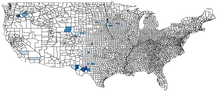
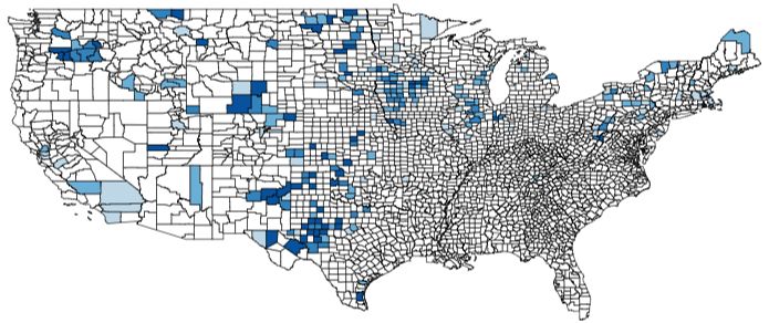
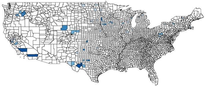
York, Massachusetts, and Connecticut. Commercial wind installations in the United States typically
consist of many individual turbines, usually ranging in capacity from 1 to 3 megawatts (MW) each. By
2019, there were over 1,500 commercial wind installations in the United States comprised of over 61,000
individual turbines. The mean and median number of turbines in a commercial wind installation as of
2019 was 42 and 21 respectively, while the mean and median capacity of commercial wind installations
was 76 and 44 MW, respectively. 4
 Figures Ia – Id document the geographic location and growth of wind energy production in the
continental United States between 1995 and 2016. The figures illustrate installed wind turbine capacity
(in MW) by county and year. In 1995, wind energy production was extremely rare and was concentrated
almost entirely in California and to a lesser degree in Texas. There were only 16 school districts in the
U.S. with wind energy installed within their boundaries at that time. By 2002, wind energy production
had begun to spread across the mid- and north-west while also expanding throughout Texas counties,
affecting 99 school districts. By 2009, there were 419 affected districts, and as illustrated in Figure 1d, by
2016, wind energy production had spread across 38 states, affecting 900 school districts, in the
continental US, the main exception being the southeastern US. 5
 There is substantial variation across states in the property tax treatment of commercial wind
energy installations. Specifically, as noted by the American Wind Energy Association (AWEA, 2017),
property tax treatment typically falls into five broad categories: 1) states that offer no special property tax
treatment, implying wind installations are taxed just like other real property; 2) states that adopted
specific formulas for taxing wind energy installations; 3) states where local jurisdictions or the state have
the authority to offer special property tax treatment; 4) states that utilize an income generation or
production tax method for wind energy installations; and 5) states that offer full or partial property tax
exemptions. 6 Furthermore, many states allow local jurisdictions to offer commercial wind installations
special tax treatment through mechanisms such as payments in lieu of taxes (PILOTS), property tax
abatements, and tax increment financing (See Appendix A for details on state-specific wind energy
policies).
 Because most school districts in the United States are independent jurisdictions with their own
taxing authority, when a wind energy installation begins operation within the boundaries of a school
district, the district will typically benefit financially from the expansion of its property tax base. However,

4
 Authors calculations based on data from the United States Wind Turbine Database (USWTDB) (Hoen et al., 2020).
5
 The primary reason that there are no wind energy installations in the Southeast is because the winds there are not
strong enough. See Appendix Figures Ia – Id for analogous maps of county-level installed wind turbine capacity per-
pupil (in kilowatts), which look very similar to main Figures Ia – Id.
6
 For more details on the property tax treatment of wind energy, see “Property Tax Treatment of Commercial Wind
Projects”, American Wind Energy Association and Polsinelli PC, 2017.

 4

the degree to which a school district benefits from a wind energy installation will depend on both the state
and local laws and ordinances governing wind energy property taxation discussed above and the
interaction of those laws with state school finance formulas. For example, during our sample timeframe,
Kansas granted a full lifetime exemption from property tax payments on wind installations and although
some wind installations made PILOT payments to hosting counties, individual school districts typically
received little to no revenue from the installations. Similarly, Wyoming has a centralized system of school
finance and thus any revenue that is generated from wind energy installations is captured entirely by the
state and redistributed through the state’s school foundation program.
 Texas provides an example where state laws governing the taxation of wind energy installations
and state school finance formulas result in a complicated system of local taxation of wind energy. School
districts in Texas may approve a tax abatement agreement which allows a temporary, 10-year limit on the
taxable value of a new wind project. These agreements, formally known as Chapter 313 agreements,
apply only to school district taxes levied for maintenance and operations (M&O). Taxes for debt service,
known as interest and sinking (I&S) fund payments are not subject to the limitation. Once a Chapter 313
agreement ends, most of the property tax revenue generated from a wind project goes back to the state
due to the Chapter 41 Recapture law in Texas (commonly referred to as Robin Hood). Because revenue
designated for I&S (debt service) is not subject to recapture and furthermore because the full increase in
assessed value due to a wind project immediately goes on a school district’s tax rolls for I&S, there is a
strong incentive for school districts in Texas to pass a bond for school capital projects and use the wind
project revenues to “subsidize” the capital improvement projects.
 Appendix A provides more information on state and local laws and ordinances governing wind
energy property taxation and how those laws interact with state school finance formulas. We present this
information for the 21 states with the largest installed capacity as of 2018. These state account for
approximately 95% of the total installed wind capacity in the nation.

III. Data
 We construct an original panel dataset that combines information on: 1) the universe of wind
energy installations in the continental United States; 2) school district revenues, expenditures, pupil-
teacher ratios, and teacher salaries; 3) student achievement, as measured by standardized test scores; and
4) census data on the socio-economic characteristics of school districts.
 National data on installed wind capacity comes from the United States Wind Turbine Database
(USWTDB). The USWTDB contains information on the date each wind turbine became operational, the
installed capacity of each turbine measured in kilowatts, and the longitude and latitude of each turbine.
We use this information to geocode every turbine to a single school district using 1995 school district

 5

boundary files maintained by the National Center for Education Statistics (NCES). 7 We then create a
panel dataset containing annual data on total installed wind capacity in each school district by aggregating
information on the capacity of every turbine in operation in a school district in a given year up to the
school district level.
 We combine the annual data on school district installed wind capacity with annual data on district
revenue and expenditures from the Local Education Agency Finance Survey (F-33) maintained by the
NCES. The F-33 surveys contain detailed annual revenue and expenditure data for all school districts in
the United States for our sample period of 1994-95 to 2016-17. In the empirical work that follows we
utilize seven revenue and expenditure outcomes: 1) local revenue, which is primarily composed of
property tax revenue; 2) state revenue, which primarily consists of state aid (grants) to local school
districts; and 3) total revenue, which is the sum of local, state, and federal revenues. 8 The expenditure
outcomes are: 1) current expenditures, which consists of expenditures for daily operations such as teacher
salaries and supplies; 2) capital outlays, which consist of expenditures for new school construction and
modernization as well as the purchase of equipment and land; 3) other expenditures, which consists of
community and adult education, interest on debt, and payments to other governments (such as the state)
and school systems (such as charter and private schools); and 4) total expenditures, which is the sum of
current, capital, and other expenditures. We divide all of these variables by enrollment to obtain per-pupil
measures and adjust them to real 2017 dollars using the Consumer Price Index (CPI).
 We merge our combined dataset with several other data sources. First, for our entire sample
period, we merge in data from the annual Common Core of Data (CCD) school district universe surveys
that provide staff counts for every school district. We then construct district-level estimates of the pupil-
teacher ratio by dividing total full-time equivalent teachers (FTE) by total district enrollment.9 Second,
we combine our dataset with data from the Special School District Tabulations of the 1990 Census on
median household income, fraction of the population at or below the poverty line, fraction white, fraction
rural, fraction age 65 or older, and fraction of adults 25 and older with a Bachelor’s degree. 10

7
 The matched USWTDB and school district boundary data include 1,916 “behind the meter” turbines. Because
these turbines are intended for on-site use rather than being part of a larger wind energy project designed for
commercial electrical generation, we drop these turbines from the analysis. We note, however, that all of our results
are robust to including them.
8
 We do not present results separately for federal revenues, because they are very small and have little to no response
to wind energy installation.
9
 Because staff counts tend to be noisy, we follow Lafortune et al. (2018) and set values of the pupil teacher ratio
that were in the top or bottom 2% of the within state-year distribution to missing.
10
 1990 district demographic data is missing for a small number of school districts. Rather than excluding these
districts, we matched school districts to counties and then replaced the missing district-level values of each variable
with their county-level equivalent.

 6

Third, we combine our dataset with information on teacher compensation. Teacher salaries are
typically a lock-step schedule based on years of experience and whether or not a teacher has a Master’s
degree. While district average teacher salaries are provided in the CCD, these conflate changes to the
teacher salary schedule with changes in hiring of new teachers that are usually paid less than the average
teacher in the district. Because information on district teacher salary schedules are not available in our
primary CCD data, we use salary schedule information from the U.S. Department of Education Schools
and Staffing Survey (SASS), which surveys a random cross-section of school districts every few years
about staffing, salaries, and other school, district, teacher, and administrator information. We focus on
district base teacher salary, which is available in every wave and particularly informative about average
teacher salaries given the high rate of teacher attrition and relatively large degree of compression in
teacher wages. Unfortunately, given the limited number of years and overlap of districts across waves, we
lose about 94 percent of our sample size.
 Finally, we use restricted-access microdata from the National Assessment of Educational
Progress (NAEP) to examine student achievement. The NAEP provides math and reading test scores in
grades four and eight from over 100,000 students in representative samples of school districts nationwide
every other year since 1990. 11 We restrict the data to the NAEP reporting sample and to public schools.
Following Lafortune et al. (2018), we then standardize students’ scores by subject and grade to the first
year each subject and grade was tested.12 We then aggregate these individual-level scores to the district-
subject-grade-year level, weighting the individual scores by the individual NAEP weight. 13
 While the NAEP provides nationally representative test score data back to the 1990s, it suffers
from small sample sizes relative to our baseline data because it is only every other year and a sample of
districts. 14 We attempt to partially remedy this drawback by merging the NAEP with a newer source of
test score data: the Stanford Education Data Archive (SEDA). For every state and for grades three
through eight, researchers at Stanford collected district test scores from 2009-2015 and standardized those

11
 The NAEP also tests in grade twelve and in other subjects such as writing, science, and economics, but we focus
on math and reading in grades four and eight because they were tested most consistently across years.
12
 Rather than providing a single score for each student, NAEP provides random draws from each student’s
estimated posterior ability distribution based on their test performance and background characteristics. We use the
mean of these five draws for each student, essentially creating an Empirical Bayes “shrunken” estimate of the
student’s latent ability.
13
 We merge the data to our primary dataset using the NCES unique district ID that is available in the Common Core
of Data (CCD) and in the NAEP data from 2000 onward. Prior to 2000, the NAEP data did not include this unique
district ID. NCES provided us with a crosswalk that they developed in collaboration with Westat to link the NAEP
district ID and the NCES district ID for those earlier years.
14
 Of particular concern is the number of treated (“wind”) districts in this reduced sample. The number of wind
districts observed in at least one year in our NAEP data (521) is only somewhat smaller than the number of wind
districts we observe in our overall sample (638). However, the more substantial loss is in the number of observations
per district, with 27% of these wind districts observed only once, and 68% observed for four or fewer years.

 7

test scores to the NAEP scaling (Reardon et al., 2018). We start with the NAEP grade 4 and 8 data from
1996-2015, and then fill in for 2009-2015 SEDA grade 4 and 8 scores for any district*year without a
NAEP score. The result is a dataset containing test scores for a sample of districts every other year from
1996-2007, and for the universe of districts every year since 2009. We standardized all scores to mean
zero and standard deviation one within year, grade, and subject.
 We restrict our main sample in several ways. First, we limit the sample to traditional school
districts, namely elementary, secondary and unified school systems, and thus drop charter schools,
college-grade systems, vocational or special education systems, non-operating school systems and
educational service agencies. 15 Second, we drop states (and thus all districts within a state) without any
wind energy installations over our sample time period of 1995-2017. 16 Third, we drop districts with
observed wind energy installations if the maximum wind capacity over our sample time frame was less
than 2 megawatts (MW). 17 Fourth because the NCES finance data tends to be noisy, we restrict the
sample to school districts with enrollment of 50 students or more in every year of our sample. Fifth, we
drop Kansas from the analysis since the state provides a full lifetime exemption from property tax
payments, and thus school districts do not benefit from wind energy installations. We similarly drop
Wyoming from the analysis because its school finance system prevents revenue generated from wind
energy installations from flowing to local school districts (see Section II). We show in Table 3 that the
results are nearly identical when we include Kansas and Wyoming.
 Our final sample consists of 11,038 school districts located in 35 states over the period 1995-
2017. 18 Among the 11,038 districts in our sample, 638 had a wind energy installation at some point
between 1995 and 2017. Table 1 presents summary statistics for the outcome measures used in our
analysis. The table presents means and standard deviations for the full sample and separately for districts
with and without wind energy installations. Districts with wind energy installations have slightly lower

15
 We also drop a small number of observations associated with the following types of educational agencies: 1)
Regional education services agencies, or county superintendents serving the same purpose; 2) State-operated
institutions charged, at least in part, with providing elementary and/or secondary instruction or services to a special-
needs population; 3) Federally operated institutions charged, at least in part, with providing elementary and/or
secondary instruction or services to a special-needs population; and 4) other education agencies that are not a local
school district.
16
 Those states are: Alabama, Arkansas, Connecticut, Florida, Georgia, Kentucky, Louisiana, Mississippi, North
Carolina, South Carolina, and Virginia.
17
 According to the Lawrence Berkeley National Laboratory, early commercial scale wind turbines had an average
capacity of between 0.7 and 1 MW. Turbine capacity has increased over time with the average capacity of a turbine
being 2.15 MW in 2016. Thus, by limiting the sample of school districts with wind energy installations to those with
2 MW or more, we are essentially eliminating districts with a single turbine. We show in Table 3 that our results are
robust to this decision.
18
 The states are: Arizona, California, Colorado, Delaware, Idaho, Illinois, Indiana, Iowa, Maine, Maryland,
Massachusetts, Michigan, Minnesota, Missouri, Montana, Nebraska, Nevada, New Hampshire, New Jersey, New
Mexico, New York, North Dakota, Ohio, Oklahoma, Oregon, Pennsylvania, Rhode Island, South Dakota,
Tennessee, Texas, Utah, Vermont, Washington, West Virginia, and Wisconsin.

 8

per-pupil local and total revenue and also slightly lower per-pupil total and current expenditures. Districts
with wind energy installations also have lower pupil-teacher ratios and base teacher salaries.
 To provide additional context about how districts with and without wind energy installations
differ, Table 1 also presents summary statistics for our outcomes and control variables at baseline. For the
outcome measures and enrollment, baseline corresponds to the 1994-95 year. For all the control variables
other than enrollment, baseline corresponds to 1989-90. Similar to the first panels of Table 1, districts
with wind energy installations have lower per-pupil local and total revenues and lower per-pupil total and
current expenditures, although the differences are larger than in the first panels of Table 1. Not
surprisingly, districts with wind installations tend to be smaller and significantly more rural. They also
tend to contain households with lower income and lower educational attainment.

IV. Methodology
 To examine the effect of wind energy installation on school district revenues, expenditures and
resource allocations, we employ a difference-in-differences identification strategy. We begin with a non-
parametric event-study specification of the following form:

 = ∑8 =−6 , + + + + , (1)

where denotes an outcome of interest for district i in state s in year t; , represents a series of lead
and lag indicator variables for when a wind energy installation became operational in district i, is a
vector of school district characteristics at baseline interacted with a linear time trend, ; is a vector of
school district fixed effects; is a vector of state-by-year fixed effects, and is a random disturbance
term. We re-center the year a wind energy installation became operational so that 0, always equals one
in the year the installation became operational in district i. We include indicator variables for 1 to 6 or
more years prior to an installation becoming operational ( −6, − −1, ) and 1 to 8 or more years after
the beginning of operation ( 1, − 8, ). Note that −6 equals one in all years that are 6 or more
years prior to the wind installation becoming operational, and 8, equals one in all years that are 8 or
more years after the beginning of operation. The omitted category is the year the installation became
operational, 0,, .
 The coefficients of primary interest in equation (1) are the ′ , which represent the difference-in-
differences estimates of the impact of wind energy installation on our outcomes of interest in each year
from −6 to 8 . The estimated coefficients on the lead treatment indicators ( −6 , . . . , −1 ) provide
evidence on whether our outcomes were trending prior to the time a wind energy installation became

 9

operational in district i. If wind energy induces exogenous increases in district revenues, expenditures
etc., these lead treatment indicators should generally be small in magnitude and statistically insignificant.
The lagged treatment indicators ( +1 , … , +8 ) allow the effect of wind energy installations on our
outcomes of interest to evolve slowly over time and in a nonparametric way. Given that treatment (wind
energy installation) occurs at the district level, in all specifications we cluster the standard errors at the
school district level.
 The inclusion of state-by-year fixed effects in equation (1) implies that our estimates are
identified off of within state variation in school district exposure to wind energy installations. Thus, our
specifications control nonparametrically for differential trends in our outcomes of interest that are
common to all districts within a state and across time. In our most parsimonious specification, 
includes 1995 district enrollment and 1990 district median income and the fraction of adults 25 and older
who have a Bachelor’s degree. We then add 1990 district fraction of the population at or below the
poverty line, fraction white, fraction 65 or older, and fraction rural. We exclude time-varying
characteristics because they could be affected by the installation of a wind energy project within a school
district (i.e., endogenous controls). Therefore, we include each characteristic interacted with a linear time
trend to allow for differential trending by districts with different baseline values of these characteristics.
 Given the substantial effect of statewide school finance reforms (SFRs) on district finances and
student achievement during our sample period, we additionally control in all models for the impacts of
SFRs. Specifically, we created an indicator variable that equals unity after the implementation of a SFR
and allow the effects of SFRs to vary by district income by interacting the SFR indicator with indicators
for terciles of the within-state 1990 median income distribution. 19
 We complement the event-study specification with a standard difference-in-differences model to
increase our precision by pooling estimates within both the pre- and post-wind energy installation
periods:

 = 0 + 1 + + + + , (2)

where is an indicator that takes the value of one in all years after a wind installation becomes
operational in district i, is a random disturbance term, and all other terms are as defined in equation
(1). The coefficient of primary interest in equation (2) is 1 which represents the difference-in-differences
estimate of the effect of treatment (wind energy installation) on our outcomes of interest.

19
 We follow the SFR codings from Brunner et al. (2020). Note that we do not include the SFR indictor separately
given it would be perfectly collinear with the state-by-year fixed effects.

 10

Finally, to account for the fact that the capacity of wind energy installations varies across
districts, in our preferred specifications we allow for continuous treatment by replacing with the
installed wind installation capacity in a district:

 = 0 + 1 + + + + , (3)

where is installed wind installation capacity in district i in state s in year t measured in kilowatts
per-pupil, is a random disturbance term, and all other terms are as defined in equation (1). 
is equal to zero for district-years with no installed wind energy. The coefficient of primary interest in (3)
is 1 which represents the effect of a one-kilowatt per-pupil increase in wind energy capacity on our
outcomes of interest.

V. Results
 We begin our analysis by examining the impact of wind energy installation on school district
revenues and expenditures using the event-study model described above. We estimate equation (1) for our
baseline sample of school districts from 1995 to 2017, and plot estimated ′ and associated 90%
confidence intervals from these regressions. Figure IIa shows that within two years of when a district first
installs wind energy, local revenues increase by approximately $1,000 per pupil. This increase in revenue
grows to between $1,500 and $1,800 per pupil several years after installation. This effect represents a
large increase given the mean local revenue in districts with installed wind energy of $6,070. Importantly,
we see no evidence of a pre-trend in local revenue prior to installation.
 Figure IIb shows similar, though slightly attenuated impacts of wind energy installation on school
district total revenue. The magnitudes are between $1,500 and $1,600 several years out. Again, the point
estimates are near zero and statistically insignificant prior to wind energy installation. Finally, given that
the other large revenue source for districts aside from local revenue is state aid, Figure IIc examines
impacts on district revenue from the State. We find small, marginally statistically significant declines in
state aid after wind energy installation of between $100 and $250 per pupil. These decreases are
consistent with the fact that many state aid formulas provide less aid to districts when local revenues are
higher. Again we see no evidence of pre-trends.
 We next examine whether these increases in revenues translate into increased expenditures, and
toward what types of expenditures districts allocate the revenue increases due to wind energy installation.
Figure IIIa shows that total expenditures per pupil increase in a similar pattern over time as total revenues
after wind energy installation, though with slightly higher magnitudes. Total expenditures increase by
between $1,500 and $2,000 per pupil several years after installation. Current expenditures increase only

 11

slightly, by between $200 and $300 per-pupil relative to a mean of just under $11,000 (Figure IIIb).
Districts spend a significant share of the revenues toward increased capital spending, which increases by
$500 and $1,000 after wind energy installation, off a mean of $1,360 per pupil (Figure IIIc). Finally, in
Figure IIId we find that other expenditures, which is simply non-capital and non-current expenditures,
increases substantially, also by between $500 and $1000 several years after wind energy installation.20
None of the figures examining district expenditures show any evidence of differential pre-trends.
 We next examine whether any of these expenditure increases lead to impacts on commonly
studied inputs to education production, for example, class size and teacher compensation. Figure IVa
shows a small, and not quite statistically significant decline in the pupil-teacher ratio, which is our
measure of class size, on the order of 0.1 pupils per teacher, relative to a mean of 13.7. This is less than a
1% decline in class size, consistent with the small (1-2%) increases in current spending. As shown in
Figure IVb there is no apparent impact on base teacher salaries, however, given the far smaller sample
using the SASS data, the results are too imprecise to gain much inference.
 One noticeable pattern in the revenue and expenditure results is that the effects of wind energy
installation grow over time. It is not immediately clear why this would be the case, as another possible
scenario could have been that the installation occurs and districts immediately and permanently reap the
tax benefits, leading to a sudden increase in the level of revenues, but no change in the trend. We examine
and rule out several possible explanations for this pattern. First, the effects on revenues and expenditures
are per-pupil, so if installations cause enrollments to decline, then this would cause the pattern that we
observe. We estimate the event-study model where the dependent variable is district enrollment and find
no impact. 21
 A second possible explanation for the growing effects over time is that we are examining the
impact relative to the year of the first wind energy installation in the district. However, 37.5% of districts
in our sample with installed wind energy install additional wind turbines over time. To examine whether
the growing effects are due to these districts with “multiple events,” we drop those districts that install
additional wind turbines in years following the initial installation. As shown in Appendix Figures III and
IV, even after dropping districts with multiple installations we still observe a pattern of rising effects over
time.

20
 We explore this result further in Section V(c), finding that it is driven primarily by Texas, and represents
payments from districts to the state. Thus, it is not a true increase in district spending, but rather a transfer of a
portion of the local revenue increases due to wind installation back to the state due the recapture design of Texas
school finance laws.
21
 See Appendix Figure II. There is evidence of a small negative pre-trend in enrollment, with no noticeable impact
post installation.

 12

The final explanation is a combination of sun-setting tax abatements and other tax rules that delay
the generation of tax revenue from wind energy installations. Many states and local jurisdictions enter
into some type of agreement in order to encourage wind development that allows wind developers a grace
period in which they do not pay (or pay significantly lower) property taxes. For example, under Iowa’s
wind energy conversion tax ordinance, a wind project is taxed at 0% during the first year of operation and
then in the second through sixth assessment years, a wind project is taxed at an additional 5% of net
acquisition costs for each year (5% in year 2, 10% in year 3, etc.) until the seventh year when taxes are
capped at 30% of net acquisition cost. While we cannot confirm empirically, laws and agreements such as
those in Iowa, appear to be the most likely reason for the growing effect over time.

A. Difference-in-Difference Estimates
 We present difference-in-differences (DD) estimates of the impact of wind energy installation in
Table 2. Results based on equation (2) with binary treatment are presented in columns 1 and 2, while
columns 3-5 present results based on equation (3) with continuous treatment. Row 1, column 1 shows that
installation causes a $1,084 per pupil increase in local revenue. Column 1 includes the basic set of
controls: baseline enrollment, 1990 median income, and 1990 fraction earning a BA or higher, all
interacted with a linear trend; and a dummy for school finance reforms interacted with terciles of the 1990
within state median income distribution. The effect is very similar, $1,005 per pupil, or 17%, relative to
the mean of $6,070, after including the expanded set of controls that adds 1990 percent poor, 1990
percent white, 1990 percent age greater than 65, and 1990 rural status, all interacted with a trend. The
effect on total revenues (column 2) is $813 (6%), and the effect on state revenues is -$111 (-2%).
 Focusing on our preferred specification in column 2, total expenditures increase by $1,031 (8%),
over $200 per pupil more than total revenues increase. The reason that total expenditures can increase
more than total revenues is that revenues in our data do not include proceeds from bond sales, while
expenditures include the spending resulting from bond sales. For example, when a district passes a bond
to finance a capital project, the proceeds do not count toward revenue, but the capital spending on the
project is included in capital, and therefore total, expenditures.
 Current expenditures increase by $133 per pupil, an increase of only 1% relative to the mean
current spending in wind energy districts of $10,948. On the other hand, capital expenditures increase by
$433 per pupil, or 32%, relative to the mean of $1,360. The larger increases in capital than operating
expenditures are perhaps unsurprising given that the school finance laws in many states require a
reduction in state aid when local revenue placed in the general fund is used to finance operating
expenditures, but do not require a reduction in state aid when local funds are placed in the capital fund

 13

and used to finance capital projects. 22 Appendix Table 1 shows that the effects on capital expenditures are
driven nearly exclusively by spending on construction of new buildings, and modernization or major
renovations to existing buildings, as opposed to purchases of land or equipment. Finally, other
expenditures increase by $465 per pupil, or 45%.
 Given the small effect on current expenditures, it is unlikely there would be large impacts on
either teacher hiring (i.e., class size) or on increasing teacher compensation. Accordingly, we find
decreases in class size of about 0.1 pupils per teacher (marginally statistically significant in column 1;
insignificant in column 2). The magnitude of the -0.09 class size estimate from column 2 represents a
0.6% percent decrease. Similarly, we find no evidence of impacts on base teacher salary, with an
insignificant point estimate of -$543 (representing a 1.6% decrease).
 While the estimates from the basic DD model with binary treatment are useful, there are two
aspects of the model that are suboptimal. First, as in the event-study analysis, the binary treatment
variable turns on when the first installation in a district occurs, and so it does not further capture the
increased capacity of subsequent installations for the 37.5% of districts with multiple installations over
time. Second, the binary treatment variable misses the important variation stemming from different wind
energy installations having very different installed capacity, while local property tax generation from
wind energy installation almost always reflects installed capacity. For example, the 10th percentile of
installed capacity per pupil in our sample among districts and years with installed wind energy is 11
KW/pupil, while the 90th percentile is 642 KW/pupil. These installations clearly have very different tax
implications, but the binary installation variable treats them identically.
 Given the limitations of the binary treatment results, in columns 3-5 we present results based on
equation (3) where we use a continuous measure of treatment, namely installed kilowatts per pupil. In
district-years without installed wind energy, this variable equals zero. Once again, the results in column 3
(basic controls) and column 4 (expanded controls) are very similar, so we focus on column 4. Row 1
shows that one additional KW/pupil of installed capacity leads to $3.78 per pupil of additional local
revenue. Column 5 multiplies the point estimate by 243, which is the mean level of installed capacity per
pupil among districts and years with installed wind energy. For example, a district with the mean level of
installed capacity per pupil experiences an increase of $918 (=3.78 x 243) per pupil in local revenue.
Total revenues increase by $3.59 with a 1 KW/pupil increase in capacity, for a $872 increase at mean
capacity. While the previous event-study and binary DD models found small, statistically significant

22
 Discussions between the authors and school district superintendents in several districts with wind energy
installations anecdotally confirm that these state laws are the primary reason districts tend to spend the money on
capital expenditures.

 14

decreases in state revenue, here we find a statistically insignificant $0.25 decrease per KW/pupil,
corresponding to a (insignificant) $61 decrease at the mean.
 In terms of expenditures, we find that total, current, capital, and other expenditures increase by
$4.81, $0.88, $2.12, and $1.81 per one KW/pupil increase, respectively, which corresponds to a $1,168
(total), $214 (current), $515 (capital), and $439 (other) increase at the mean level of installed capacity.
Turning next to pupil-teacher ratio, to aid in interpretation for the continuous DD we multiply the point
estimates in columns 3 and 4 by 1,000. Thus, a 1 KW/pupil increase in capacity causes a marginally
significant decrease of 0.00015 pupils per teacher (presented as -0.15 in column 4 of Table 2), which is
equivalent to 0.04 pupils per teacher at the mean. While this is marginally significant, it is essentially
zero. Note that the increase in current expenditures is approximately 2% while the pupil teacher ratio
decreases by substantially less than 2%. Thus, one interpretation of these findings is that districts are not
spending the increases in current expenditures on hiring new teachers, although we do not have enough
statistical precision to be confident in this claim. We conservatively interpret these effects as consistent
with the prior results that there are small impacts on current spending, and near zero impacts on class size
reduction. As in the previous models, there is no impact on teacher salary. However, using the continuous
DD model the zero effect at the mean capacity is quite precisely estimated with a point estimate of $59
and standard error of $73, allowing us to rule out a positive effect on salaries greater than approximately
$200.
 In summary, districts that install wind energy see large increases in local revenues that are only
minimally offset by reductions in state aid, leading to large increases in total revenue. The districts spend
these increases primarily on capital outlays, and on other, non-current and non-capital expenses, which
we examine in further detail below.

B. Sensitivity Analysis
 In this section, we conduct seven sensitivity checks to examine the robustness of our results to
decisions about the way we construct our sample and implement the difference-in-differences analysis.
We proceed with our preferred specification, which is the continuous DD model with the expanded set of
controls (Table 2, column 4). The first row of Table 3 replicates our baseline preferred model for
comparison purposes.
 In our first check, we include the eleven states, primarily in the South census region, with no
installed wind energy during our sample period. In the second check, we include the two states, Kansas,
and Wyoming, which we removed because their laws prevent wind energy tax revenue from being
directed toward local school districts. In our third check, we include districts with a maximum installed

 15

wind energy capacity during our sample period of less than 2 MW. In all of these checks, the results are
nearly identical to our baseline estimates.
 In our fourth check, we restrict to counties with installed wind energy. In our baseline sample, we
include counties with no installed wind energy if they are in a state with installed wind energy, even
though these counties may be quite different from counties in that state with installed wind energy. This
check is meant to create a control group of school districts without installed wind energy that looks more
like the treated school districts, by drawing within state comparisons (due to the state-by-year fixed
effects) between school districts with wind energy and those without, but that are in counties with wind
energy. In spite of the sample size dropping from 218,851 district-years to 42,767, the point estimates are
very similar.
 Given that treated districts tend to be smaller than untreated districts, in our fifth check we drop
large untreated districts. Specifically, we drop districts with no installed wind energy that have enrollment
greater than the 90th percentile of enrollment among treated districts. The estimates are nearly identical to
those using our preferred specification. In our next specification check we use propensity score weighting
to weight higher those non-wind districts that are observationally similar to districts with wind energy. 23
Once again, the estimates using the propensity score weighting are very similar to our baseline results.
 Finally, to further account for any differences between districts with high versus low (or zero)
installed wind energy capacity, we use average wind speed as an instrument for installed capacity.
Specifically, we use the average wind speed at each school district’s centroid at a 100-meter height during
the period 2007-2013. 24 We instrument for installed capacity with the interaction of our time-invariant
wind speed measure with a dummy for having installed wind energy in that year. This instrumental
variables strategy produces results that are very similar to those from our main analysis, the only
difference being that the reduction in state aid is larger and significant ($0.48 relative to $0.25), though
still small relative to the increase in local revenues.

23
 Specifically, we run a logit regression of a dummy for a district having wind energy on 1990 rural status, median
household income, fraction BA or higher, fraction age 65 or older, fraction white, fraction poor, and baseline
enrollment. We then create a propensity score from that regression, which is simply the predicted probability that a
district has wind energy. Finally, we create inverse propensity score weights, equal to wind / pscore + (1-wind)/(1-
pscore).
24
 These data come from the Wind Integration National Dataset (WIND) Toolkit (Draxl, et al., 2015). The 100-meter
height reflects typical wind turbine height, and the period 2007-2013 is the period of available data. The first stage
F-statistic for our IV regression is 127. Appendix Table 2 shows all of our main results (i.e., binary and continuous
difference-in-differences, with and without the expanded controls) using the wind speed instrument, again showing
very similar effects.

 16

C. State Heterogeneity and Other Expenditures
 As described in Section II, there is substantial heterogeneity not only in state laws regarding
taxation of wind energy installation, but also in school finance laws. The interaction of these two quite
heterogeneous sets of laws could create very different impacts of wind energy installation in different
states. While the average national effect of wind energy installation we have presented is of primary
interest, it is also important to understand whether our results are driven in part by any particular state. An
obvious state to consider in our case is Texas, which is by far the largest producer of wind energy in the
country, comprising 28% of installed capacity in our national sample. 25 In this section we explore whether
and to what extent our national results are driven by Texas.
 Table 4 presents effects of wind energy installation on revenues and expenditures using our
preferred specification (continuous DD with expanded controls) for our national sample (baseline –
column 1), Texas only (column 2), and our national sample without Texas (column 3). We find much
larger impacts in Texas than in the national sample on local revenue and total revenue of $7.78 and $8.04
per pupil from a 1 KW/pupil increase in capacity. In column 3, where we drop Texas, the point estimates
for local and total revenue are substantially smaller at $2.33 and $1.99 respectively. Also, in column 3,
the reduction in state revenue increases slightly in magnitude and becomes marginally significant, though
it is still quite small ($-0.48). Total, current, capital, and other expenditures in Texas increase by $10.03,
$0.88, $4.33, and $4.82, respectively. The effect on current is identical to the baseline estimates, but the
other three outcomes have much larger point estimates (i.e., an even smaller share of the expenditure
increase is devoted toward current spending). Importantly, Texas completely drives the large increases we
observed in other expenditures: without Texas, the coefficient on other expenditures drops from $1.81 to
$0.70 and becomes statistically insignificant.26
 The large impacts in Texas on other expenditures begs the question of what specific type of
expenditure is driving that effect. In the bottom rows of Table 4, we show effects on the expenditure sub-
categories that comprise other expenditures. The effect on other expenditures in Texas comes almost
completely from payments to the state government, with a small increase as well in interest payments on
debt. The large increase in payments to the state government is a function of the Texas school finance
laws, whereby property tax revenue from districts with high property tax bases is recaptured by the state
and redistributed to districts with low property tax bases, a policy commonly referred to as Robin Hood.
The large impact on other expenditures, therefore does not actually reflect school district spending on any
productive education input, but rather a different form of state aid reduction. This implies that while the

25
 The next largest, California, produces only 9% of installed wind capacity in our national sample.
26
 The effect on pupil-teacher ratio without Texas is a statistically significant 0.28 reduction, which is larger than our
baseline estimate, but still very small. The effect on teacher salary (0.309) is still small and statistically insignificant.

 17