Search for Stellar Streams in The Galactic Halo From Gaia DR2, GALAH DR2, RAVE DR5 and LAMOST DR4 Data
←
→
Page content transcription
If your browser does not render page correctly, please read the page content below
EPJ Web of Conferences 240, 07012 (2020)                                        https://doi.org/10.1051/epjconf/202024007012
SEAAN Meeting 2019

          Search for Stellar Streams in The Galactic Halo From Gaia
          DR2, GALAH DR2, RAVE DR5 and LAMOST DR4 Data

          Ni Made Kartika Wijayanti1,∗ , Mochamad Ikbal Arifyanto2,∗∗ , and Nur Annisa1
          1
            Astronomy Study Program, Faculty of Mathematics and Natural Sciences, Institut Teknologi Bandung,
            Indonesia
          2
            Astronomy Research Division, Faculty of Mathematics and Natural Sciences, Institut Teknologi Ban-
            dung, Indonesia

                         Abstract. Stellar streams are stars which are trapped in the same potensial
                         caused by dynamical resonance or tidal force. We√aim to analyze kinematic sub-
                         structures (streams) in the Galactic halo by V vs U 2 + 2V 2 planes of Arifyanto
                         & Fuchs. We crossmatched data from Gaia DR2, GALAH DR2, RAVE DR5
                         and LAMOST DR4 based on positions. We have 3D kinematics and metallicity
                         data of halo stars selected from kinematics criteria from ratio of probability of
                         thick disk (TD) over halo (H) less than 0.01. Substructures are detected by
                         using wavelet transformation and corrected using √ 15 Monte Carlo simulations.
                         We obtained four kinematic structures on V vs U 2 + 2V 2 plane which two of
                         them are associated to BB17-1 and BB17-2 streams. All the streams had a high
                         probability from the extragalactic origin.

          1 Introduction
          There are two scenarios of galactic formation. First is monolithic collapse by Eggen, Lynden-
          Bell, and Sandage [1]. In monolithic collapse, a galaxy is formed from the same protogalaxy
          cloud which collapsed and every part of galaxy, such as bulge, disk, and halo, is formed at the
          same time. The second one is hierarchical scenario [2]. In this scenario, each part of galaxy
          is formed from different clouds then merge into one and forming a galaxy. This scenario can
          explain that stars in bulge, disk, and halo have different typical age. Hierarchical scenario
          is supported by a proof that Sagittarius dwarf spheroidal (Sgr dSph) deformed because of
          tidal force from Galactic center [3]. Some globular clusters such as M54, Arp2, Terzan7, and
          Terzan8 are suggested that came from Sgr dSph. Helmi and White [4] also showed that local
          stellar halo is builded by disrupted satellites.
              Eggen introduced "moving group" as stars from an open cluster or from the same protostar
          cloud. The stars then escaped from the system so they are detected as a group of stars with the
          same velocity [5]. In 1978, Eggen introduced "retrograde group," stars that expected came
          from ω Centauri cluster [6]. Metalicity and age of stars in retrograde group are broad in range
          so this suggests that ω Centauri was a galaxy and stripped into Milky Way [7].
              There are two types of streams: dynamical stream and tidal steam [8]. Stars that trapped
          into the same dynamical resonance, such as bar resonance and spiral arm resonance, is called
               ∗ e-mail: kartika.wijayanti@students.itb.ac.id
              ∗∗ e-mail: ikbal@as.itb.ac.id

    © The Authors, published by EDP Sciences. This is an open access article distributed under the terms of the Creative
    Commons Attribution License 4.0 (http://creativecommons.org/licenses/by/4.0/).
EPJ Web of Conferences 240, 07012 (2020) https://doi.org/10.1051/epjconf/202024007012
SEAAN Meeting 2019
dynamical stream. Stars that came from the same bounded object, such as satellite galaxy,
can escaped from the system and enter the Milky Way forming tidal stream. Search for stellar
streams are using star grouping in velocities space or integral of motion space. Dehnen [9],
Skuljan [10], and Kushniruk et al. [11] use U vs V space for streams in Galactic disk. Several
well-known streams are Hyades, Pleiades, and Sirius. These streams were thought to be
originated from disrupted open cluster but their isochrone showed possibility
√ of dynamical
resonant origin [12]. Arifyanto & Fuchs [13] and Klement [8]√use V vs U 2 + 2V 2 space to
identify streams in disk. Bajkova and Bobylev [14] use V vs U 2 + 2V 2 space for searching
streams in Galactic halo. Another integral of motion spaces for searching streams are Vaz vs
V∆E ([15], [16]), Lz vs L⊥ [8], and Lz vs E ([17], [18]). √
In this work, stellar streams are searched using V vs U 2 + 2V 2 planes. U is velocity
vector
√ towards Galactic center, V is velocity vector in the direction of rotation of Galaxy and
U + 2V 2 is related to eccentricity of star’s explained in Section 3.
2
2 Data
To get velocities, we use parallax and proper motion data from Gaia DR2 [19] and radial
velocity data from LAMOST DR4 [20], RAVE DR5 [21], and GALAH DR2 [22]. LAMOST
DR4, RAVE DR5, and GALAH DR2 are crossmatched into Gaia DR2 data based on star’s po-
sition with 0.8” radius. We select solar neighborhood stars with galactocentric radius within
7 to 10 kpc and distance from galactic plane Z < 5 kpc. We also eliminate stars with total
velocity more than 580 kms−1 which is the Galactic escape velocity [23]. The selected stars
are transformed to UVW velocities using matrix from [24] as shown in equation 1.
+ cos α cos δ − sin α − cos α sin δ Vr U
U
V = T. + sin α cos δ + cos α − sin α sin δ kµα /$ + V
,
(1)
+ sin δ + cos δ kµδ /$
W 0 W
where T is transformation matrix from galactic coordinates to equatorial coordinates, α and
δ are equatorial coordinates, Vr is radial velocity, k is 4,74057 to transform all the units into
kms−1 , µα and µδ are proper motion in equatorial coordinates, and $ is parallax of the stars.
We use Sun’s velocity component is (U, V, W) = (11.1, 12.24, 7.25) kms−1 [25].
Galactic halo stars are selected kinematically as performed in [26]. We use probability
of thick disk over halo T D/H = XXTHD ffTHD < 0.01 to reduce contamination from thick disk.
Each XT D and XH is fraction number of thick disk and halo respectively. Each fT D and fH is
Gaussian distribution function for stars in thick disk and halo respectively. The function of
Gaussian distribution of 3D stellar kinematics is
1 U2 (V − Vasym )2 W2
f = exp − − − , (2)
(2π) σU σV σW
3/2 2
2σU 2
2σV 2σ2W
where σU , σV , and σW is velocity dispersions of each stellar population and Vasym is asym-
metric drift relative to LSR. Value of σU , σV , σW , and Vasym in equation 2 is shown in Table
1.
3 Search Method
√ √
To find streams, we identify groupings on V vs U 2 + 2V 2 space. Value of U 2 + 2V 2
represents eccentricity of the star. Using Taylor expansion around 1/R and 1/R0 until second
2EPJ Web of Conferences 240, 07012 (2020) https://doi.org/10.1051/epjconf/202024007012
SEAAN Meeting 2019
Table 1: Fraction number and characteristics of Gaussian distribution for stars in thick disk
and halo.
σU σU σU Vasym
X
kms−1
Thick Disk (TD) 0.09 67 38 35 -46
Halo (H) 0.0015 160 90 90 -220
√
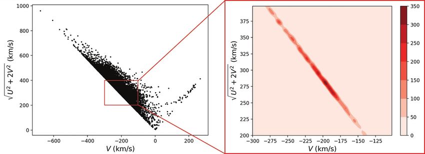
Fig. 1. Sample data distribution on V vs U 2 + 2V 2 space (left panel). Wavelet transforma-
tion of the data in range of the red box is shown on the right panel.
q
order, Dekker’s definition of angular velocity Ω(R) = 1 dΦ
R dR [27], and energy of stars in the
guiding center E0 = Φ(R0 ) + 2 R0 Ω (R0 ),
1 2 2
Arifyanto & Fuchs [13] got eccentricity of stars is
v
t 2 κ02 2
u
u
U + Ω2 V
s
2(E − E0 )
e= = 0
. (3)
R20 κ02 R20 κ02
κ02 √
For flat rotation curve, = 2 and R20 κ02 = 2V 2 so e ∝ U 2 + 2V 2 .
Ω20
√
Distribution of the data on V vs U 2 + 2V 2 space is shown on left panel of Fig. 1. The
groupings on this distribution are found using Mexican-hat wavelet transform from Skuljan
[10]. Wavelet is a powerful way to extract signal from data distribution. We divide the data
into several bins and calculate the wavelet coefficient of each bin using equation 4. For a
two-dimensional distribution f (x, y) at any point (ξ, η), the function of wavelet coefficient is
Z ∞Z ∞ x − ξ y − η
w(x, y) = f (x, y)ψ , dxdy, (4)
−∞ −∞ a a
where ψ is the analysing wavelet function. Herep we use two-dimesional Mexican hat
ψ(d/a) = (2 − (d/a)2 ) exp(−d2 /(2a2 )), where d = x2 + y2 or the distance from bin to the
data. The bin is square with 2 kms−1 width and scale parameter a is 4 kms−1 . The result of
the transformation is shown in√right panel of Fig. 1. We show significant groupings in range
V = [−300, −100] kms−1 and U 2 + 2V 2 = [200, 400] kms−1 because otherwise is relatively
smooth.
The detected groupings are corrected using Monte Carlo simulation to reduce the statistic
fluctuation. We generate 15 simulations, each simulation has the same number of stars as
3EPJ Web of Conferences 240, 07012 (2020) https://doi.org/10.1051/epjconf/202024007012
SEAAN Meeting 2019
Fig. 2. Four groupings found after cleaning the data using Monte Carlo simulation.
our data. The synthetic data from simulation have the same Gaussian distribution as Galactic
halo. Each simulation is treated the same as the data to get the wavelet transformation with
the same size of bin. Each simulation is subtracted with transformed data. The mean of each
substraction is shown in Fig. 2.
Table 2: Streams found and associated streams.
Coordinates of
Coordinates
Streams found Associated streams associated streams
kms−1 kms−1
A (-186,266) BB17-1 [14] (-170,250)
B (-196,280)
C (-207,296)
D (-227,325) BB17-2 [14] (-220, 330)
4 Results
In this work, we found four streams or groupings as shown in Fig. 2 and Table 2. We labeled
the groupings as A, B, C, and D. We suggest that two of them, A and D, are associated to
BB17-1 and BB17-2, high velocity streams in Galactic halo by Bajkova & Bobylev [14].
Bajkova & Bobylev found three streams named BB17-1, BB17-2, and BB17-3. BB17-1
and BB17-2 are correlated to VelHel-6 and VelHel-7 streams by Helmi et al. [17]. Several
streams found by Helmi et al., named VelHel-1, 2, 3, 4, 5, 8, and 9, have positions close to ω
Centauri globular cluster. Properties of this cluster support the idea of ω Centauri probably
was a galaxy and stripped into Milky Way. ω Centauri have a high mass (∼ 7 × 10⁶ M ),
4EPJ Web of Conferences 240, 07012 (2020) https://doi.org/10.1051/epjconf/202024007012
SEAAN Meeting 2019
flattened shape or tidal features, wide range of abundance and age, and retrograde orbit [7].
Other streams in Galactic halo may be the result of dwarf satellite galaxy. On the next work,
we will analyze more about origin of these streams.
Acknowledgement
The authors present results from the European Space Agency (ESA) space mission Gaia
(https://www.cosmos.esa.int/gaia), processed by the Gaia Data Processing and Analysis
Consortium (DPAC). We also used data from GALAH (https://galah-survey.org/), RAVE
(https://www.rave-survey.org), and Guoshoujing Telescope the Large Sky Area Multi-Object
Fiber Spectroscopic Telescope LAMOST (http://dr4.lamost.org/).
References
[1] O.J. Eggen, D. Lynden-Bell, A.R. Sandage, ApJ 136, 748 (1962).
[2] L. Searle, R. Zinn, ApJ 225, 357 (1978).
[3] R.A. Ibata, G. Gilmore, M.J. Irwin, Nature 370, 194-196 (1994).
[4] A. Helmi and S.D.M. White, MNRAS 307, 495-517 (1999).
[5] O.J. Eggen, AJ 112, 1595 (1996).
[6] O.J. Eggen, ApJ 221, 881-892 (1978).
[7] S.R. Majewski, R.J. Patterson, D.I. Dinescu, W.Y. Johnson, J.C. Ostheimer, W.E. Kunkel,
C. Palma, arXiv 9910278 (1999).
[8] R. Klement, B. Fuchs, H.W. Rix, ApJ 685, 261-271 (2008).
[9] W. Dehnen, AAS 115, 2384 (1998).
[10] J. Skuljan, J.B. Hearnshaw, P.L. Cottrell, MNRAS 308, 731-740 (1999).
[11] I. Kushniruk, T. Schirmer, T. Bensby, A&A 608, A73 (2017).
[12] B. Famaey, A. Siebert, A. Jorissen, A&A 483, 453-459 (2008).
[13] M.I. Arifyanto & B. Fuchs, A&A 449, 533-538 (2006).
[14] A.T. Bajkova & V.V. Bobylev, Astron. Lett. 44, 193-201 (2018).
[15] C. Dettbarn, B. Fuchs, C. Flynn, M. Williams, A&A 474, 857-861 (2007).
[16] R.J.Klement, Astron Astrophys Rev 18, 567-594 (2010).
[17] A. Helmi, et al. 2017. A&A, 598, A58
[18] H. Li, C. Du, S. Liu, T. Donlon, H.J. Newberg, ApJ 874, 1 (2019).
[19] Gaia Collaboration, A&A 616, A1 (2018a).
[20] A.L. Luo, Y.H. Zhao, G. Zhao, VizieR Online Data Catalog, V-153 (2018).
[21] RAVE Collaboration. AJ 153, 75 (2017).
[22] GALAH Collaboration, MNRAS 478, 4513-4552 (2018).
[23] Monari, G. et al . 2018. A&A 616, L9.
[24] D.R. Johnson & D.R. Soderblom, AJ 93, 864-867 (1986).
[25] R. Schönrich, J. Binney, and Walter Dehnen
[26] T. Bensby, S. Feltzing, M.S. Oey, A&A 562, A71 (2014).
[27] E. Dekker, Phys. Rep. 24, 5 (1976).
5You can also read