Forecast of Shanghai Port Throughput Based on ARIMA
←
→
Page content transcription
If your browser does not render page correctly, please read the page content below

IOP Conference Series: Earth and Environmental Science

PAPER • OPEN ACCESS

Forecast of Shanghai Port Throughput Based on ARIMA
To cite this article: JianChen Zhang 2021 IOP Conf. Ser.: Earth Environ. Sci. 831 012042

View the article online for updates and enhancements.

                               This content was downloaded from IP address 46.4.80.155 on 07/10/2021 at 14:56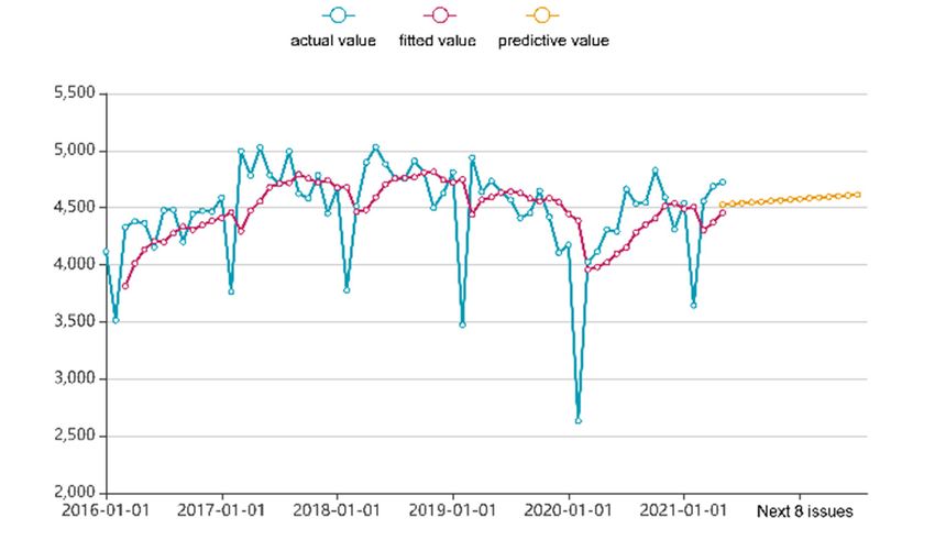
AEECE 2021                                                                                                     IOP Publishing
IOP Conf. Series: Earth and Environmental Science 831 (2021) 012042                        doi:10.1088/1755-1315/831/1/012042

Forecast of Shanghai Port Throughput Based on ARIMA

                     JianChen Zhang1, *
                     1
                         College of Transport & Communications, Shanghai Maritime University
                     *
                         Corresponding author: 202030610111@stu.shmtu.edu.cn

                     Abstract: The ARIMA model analyzes and predicts the total port throughput of Shanghai Port
                     since its inception in 2016. The mathematical model is used to predict the port throughput, which
                     provides a scientific basis for its formulation of port development strategies and is of great
                     significance to ensure the sustainable development of the port.

1. Introduction
As the largest port in the world at present, Shanghai Port plays an important leading role in the
development of the country and the world's shipping industry. Therefore, scientific prediction of the
Shanghai Port throughput trend is of great significance to the adjustment and optimization of research
development strategies. Zhou[1]scientifically analyzed and forecasted the container throughput of
Ningbo Port; Han and Xu[2] carried out forecast research on the cargo throughput of Qingdao Port based
on ARIMA and GM models; Tang[3] analyzed the influencing factors of port throughput, and then used
the systematic clustering method to determine the typical factors. Using the typical factors as
independent variables, he applied the multiple linear regression analysis method to establish the port
throughput typical factor forecasting model; Wang[4] compared the time series model forecasting method,
regression model forecasting method and gray model forecasting method, and summarized the
characteristics and application of each method; Gui[5] During the epidemic period, the gray model was
used to predict the throughput of Shanghai Port, and based on the data results, the development
countermeasures and thinking of Shanghai Port were put forward.
    Based on existing research, this paper uses the ARIMA model to predict the total throughput data of
Shanghai Port since 2016, and puts forward a scientific reference for the development strategy of
Shanghai Port in the new era.

2. ARIMA model
The basic idea of ARIMA is: The observed value of the predicted object is to obtain random data in
chronological order. These observations have a certain dependence, and this dependence is the past
change law of a certain variable. Use this law to establish a certain The mathematical model of this
model, once identified, can predict the future value from the past and present values of the time series.
If the processed ARIMA model is accepted, it can be applied to the previous sample data and current
data in the time series to predict future data. Based on time series theory, a series of related indicators
can be predicted. The modeling of time series belongs to the category of dynamic economics and can be
applied in a very wide range of fields, for example, in the prediction of future development of enterprises.
The use of the ARIMA model requires the stability of the data. The stationarity requires that the fitted
curve obtained through the sample time series can continue to be "inertial" along the current state for a
period of time in the future; the stationarity requires the mean and sum of the series The variance does
not change significantly; the greater the variance, the greater the data fluctuation. The variance
              Content from this work may be used under the terms of the Creative Commons Attribution 3.0 licence. Any further distribution
              of this work must maintain attribution to the author(s) and the title of the work, journal citation and DOI.
Published under licence by IOP Publishing Ltd                          1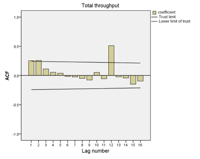
AEECE 2021 IOP Publishing
IOP Conf. Series: Earth and Environmental Science 831 (2021) 012042 doi:10.1088/1755-1315/831/1/012042
calculation formula is shown in the following formula:
2
( X ) 2
(1)
N
Among them: is the overall variance, X is the variable, is the overall mean, N is the overall
2
number of cases.
When the data fluctuates greatly, the difference method can be used to process the data to convert
the non-stationary series into a stationary series.
The ARIMA (p, d, q) model is called Autoregressive Integrated Moving Average Model, p is the
autoregressive term, q is the number of moving average terms, and d is the time when the time series
becomes stationary. Number of differences made. The so-called ARIMA model refers to a model
established by transforming a non-stationary time series into a stationary time series, and then regressing
the dependent variable only on its lag value and the present value and lag value of the random error term.
The ARIMA model includes autoregressive process (AR), moving average process (MA),
autoregressive moving average process (ARMA) and ARIMA process according to whether the original
sequence is stable or not and the parts contained in the regression are different.
The autoregressive process (AR) describes the relationship between the current value and the
historical value, and uses the historical time data of the variable itself to predict itself. The autoregressive
model must meet the requirements of stationarity. The formula definition of the p-order autoregressive
process:
p
yt i yt i t (2)
i 1
Among them: yt is the current value, is the constant term, p is the order, i is the autocorrelation
coefficient, and t is the error.
The moving average model (MA) focuses on the accumulation of error terms in the autoregressive
model. The moving average method can effectively eliminate the random fluctuations in the forecast.
The formula definition of the q-order autoregressive process:
q
yt t i t i (3)
i 1
Autoregressive moving average model (ARMA), a combination of autoregressive and moving
average, the formula is defined as follows, we can get the following formula, when we get the ARMA
model, we only need to specify three parameters (p, d, q), d is the order, d=1 is the first-order difference,
d=2 is the second-order difference, and so on.
p q
yt i yt i t i t i (4)
i 1 i 1
The time series modeling steps mainly include: First, plot the acquired series data and observe
whether it is a stationary time series; if it is a stationary series, no data processing is required, if it is a
non-stationary series, the d-order difference should be carried out to make It is transformed into a
stationary series, d in the ARIMA(p,d,q) model is the difference order; secondly, find the autocorrelation
coefficient ACF and partial autocorrelation coefficient PACF of the stationary series, and the
autocorrelation graph and partial autocorrelation coefficient Analyze the correlation graph to obtain p
and order q, thereby obtaining the ARIMA model; finally, the obtained ARIMA model is tested.
3. Model prediction
This article obtains the total throughput data from 2016 to May 2021 from SIPG's official website, and
uses the ARIMA model to make predictions based on the data.
2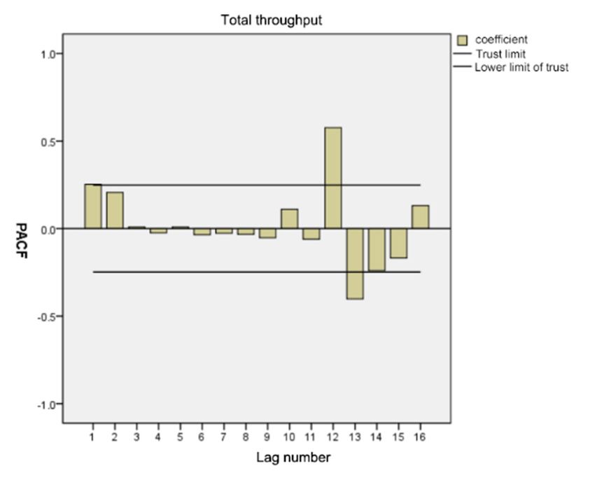
AEECE 2021                                                                                 IOP Publishing
IOP Conf. Series: Earth and Environmental Science 831 (2021) 012042    doi:10.1088/1755-1315/831/1/012042

3.1. Model ordering
According to the time series diagram of the initial data (Fig. 1), the data fluctuates greatly from 2016 to
May 2021, and the series is non-stationary. Therefore, the difference method needs to be used to obtain
a stationary series (Fig. 2).

                        Fig. 1 Throughput timing chart from 2016 to May 2021

                            Fig. 2 Timing diagram after first-order difference

3.2. Model estimate
According to the stationarity characteristics of the series, by observing the autocorrelation coefficient
graph (Fig. 3) and the partial autocorrelation coefficient graph (Fig. 4), it is determined to establish the
ARIMA (0, 1, 1) model,

                                                      3
AEECE 2021 IOP Publishing
IOP Conf. Series: Earth and Environmental Science 831 (2021) 012042 doi:10.1088/1755-1315/831/1/012042
Fig. 3 Autocorrelation coefficient graph
Fig. 4 Partial autocorrelation coefficient diagram
The model fitness parameters are shown in Table 1.
Table 1. Model fitness parameters
Model fitness
Percentiles
Fitness
average minimummaximum
statistics 5 10 25 50 75 90 95
Stationary R-
0.338 0.338 0.338 0.338 0. 338 0.338 0.338 0.338 0.338 0.338
squared
R-squared 0.011 0.011 0.011 0.011 0.011 0.011 0.011 0.011 0.011 0.011
4AEECE 2021 IOP Publishing
IOP Conf. Series: Earth and Environmental Science 831 (2021) 012042 doi:10.1088/1755-1315/831/1/012042
RMSE 423.988 423.988 423.988 423.988 423.988 423.988 423.988 423.988 423.988 423.988
Map 6.985 6.985 6.985 6.985 6.985 6.985 6.985 6.985 6.985 6.985
MaxAPE 66.593 66.593 66.593 66.593 66.593 66.593 66.593 66.593 66.593 66.593
MAE 282.399 282.399 282.399 282.399 282.399 282.399 282.399 282.399 282.399 282.399
MaxAE 1752.651 1752.651 1752.651 1752.6511752.6511752.6511752.6511752.6511752.6511752.651
Standardized
12.294 12.294 12.294 12.294 12.294 12.294 12.294 12.294 12.294 12.294
BIC
3.3. Residual test
Table 2 shows the Q statistic information of the model, including the statistic value and the p-value. The
ARIMA model requires the model residuals to be white noise, that is, the residuals have no
autocorrelation, and the white noise test can be performed by the Q statistic test (Null hypothesis: The
residual is white noise);
For example, Q6 is used to test whether the first 6-order autocorrelation coefficients of the residuals
meet white noise. Usually, the corresponding p value is greater than 0.1, indicating that the white noise
test is satisfied (otherwise, it means that it is not white noise). In common cases, it can be directly
analyzed for Q6. can;
If the white noise assumption is rejected (pAEECE 2021 IOP Publishing
IOP Conf. Series: Earth and Environmental Science 831 (2021) 012042 doi:10.1088/1755-1315/831/1/012042
Fig.5 Fitting and prediction of total throughput model
ARIMA (0, 1, 1) predicts the total throughput of the next 15 periods as shown in Table 3, showing a
steady increase.
Table 3. forecast data
Category Predictive value
1 4527.794
2 4533.934
3 4540.075
4 4546.215
5 4552.356
6 4558.496
7 4564.637
8 4570.778
9 4576.918
10 4583.059
11 4589.199
12 4595.34
13 4601.48
14 4607.621
15 4613.761
4. Development countermeasures
Do fine enterprise management and promote technological innovation. Further optimize and improve
the management system and mechanism, make every effort to promote the application of key
technologies such as big data and artificial intelligence, vigorously promote the construction of port
automation and the automation of traditional container terminals, and improve port operation efficiency
and international competitiveness.
Build a shipping service industry chain and build a high-end shipping service market. Actively
participate in the global competition for the allocation of international shipping resources, deepen the
opening of the shipping service industry to a greater extent, conform to international shipping policies,
and attract high-end shipping service elements.
With the help of free trade ports, the shipping finance industry will be developed. Shanghai Free
6AEECE 2021 IOP Publishing
IOP Conf. Series: Earth and Environmental Science 831 (2021) 012042 doi:10.1088/1755-1315/831/1/012042
Trade Port is a functional system that integrates research and development related to advanced
manufacturing, high-end assembly and assembly, offshore trade, and re-export trade. It can not only
promote the prosperity of trade, but also promote the development of a large number of modern service
industries such as ship supply, shipping finance, insurance and maritime law.
5. Conclusions
Taking into account the availability of data, this paper builds a prediction model based on the total
throughput data of Shanghai Port from 2016 to May 2021. The results show that the ARIMA (0, 1, 1)
model can accurately predict and can be used by related departments. The formulation of policy
measures and the adjustment of development strategies provide a scientific basis.
References
[1] Zhou FengTing. Analysis and Forecast of Ningbo Port Container Throughput[J].Journal of Science
& Technology Economics,2018,26(04):207.
[2] Han Yilun, Xu Xinxin.Research on Qingdao Port Cargo Throughput Forecast Based on ARIMA and
GM Models[J].Waterways and Ports,2019,40(02):241-248.
[3] Tang Simin, Lan Peizhen, Zhu Jingjun. Prediction model of typical factors of port
throughput[J].Journal of Shanghai Maritime University,2018,39(02):41-44+102.
[4] Wang Zhuo, Gao Lu. Research on Port Container Throughput Forecast Method[J].Journal of
Shanghai University of Engineering Science,2020,34(02):201-206.
[5] Gui Dehuai, Zhang Xianxuan. Analysis of Shanghai Port Container Throughput Forecast Based on
Grey Forecasting Model[J].Journal of Chuzhou Vocational and Technical College,
2020,19(03):33-36+40.
7You can also read