Sentinel-1 Toolbox SAR Basics Tutorial - Issued March 2015 Updated November 2019 Updated January 2021 Luis Veci Andreas Braun - STEP
←
→
Page content transcription
If your browser does not render page correctly, please read the page content below
Sentinel-1 Toolbox

                                  SAR Basics Tutorial
                                                         Issued March 2015
                                                    Updated November 2019
                                                      Updated January 2021

                                                                          Luis Veci
                                                                     Andreas Braun

Copyright © 2020 Array Systems Computing Inc. http://www.array.ca/
                        http://step.esa.int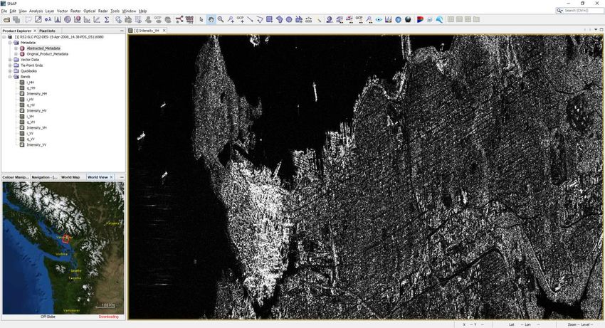
SAR Basics Tutorial

SAR Basics Tutorial
The goal of this tutorial is to provide novice and experienced remote sensing users with step-by-step
instructions on working with SAR data with the Sentinel-1 Toolbox.

For further details on operator parameters and algorithmic descriptions, please refer to the online help
available within the software.

In this tutorial you will calibrate, multilook, speckle filter, and terrain correct SAR data products.

Sample Data
For this tutorial, we will use the Vancouver Fine Quad2 SLC dataset. Vancouver in British Columbia is the
third largest metropolitan area in Canada located on the Pacific coast.
Sample data for RADARSAT-2 Fine Quad-Pol products supplied by MDA can be found at:
▪ https://mdacorporation.com/geospatial/international/satellites/RADARSAT-2/sample-data/

Download and unzip the Vancouver_R2_FineQuad2_HH_VV_HV_VH_SLC product (217.37 MB).

Open a Product
Step 1 - Open a product: Use the     Open Product button in the top toolbar and browse for the
location of the Vancouver Fine Quad RADARSAT-2 product.

Select the product.xml file and press Open Product (Figure 1. If your product is contained within a zip
file, the Toolbox will also be able to open the product simply by selecting the zip file. If you encounter
problems with opening data, select a specific reader under File > Import > SAR sensors.

                                         Figure 1: Open the product.xml

                                                                                                             2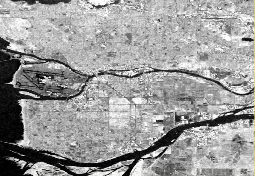
SAR Basics Tutorial

In the Products View you will see the opened product which consists of Metadata, Vector Data, Tie-
Point Grids, Quicklooks and Bands (which contains the actual raster data, organized by polarization).

Double-click on the Intensity_VH band to view the raster data. The product is a RADARSAT-2 Single
Look Complex (SLC) data product which means that it is stored and displayed in slant geometry (as
measured by the side-looking sensor) and has not been multilooked. This means that the data can
appear stretched in the azimuth direction (y axis) and contain a lot of noise.

                                           Figure 2: Product view

You can use the World View or World Map (to see its full extent on a base map) or open the Quicklook
for a preview of the dataset in an RGB color representation. If you miss any items in your user interface,
you can activate them in the menu under View and Tool Windows.

You can find information on the product under Metadata > Abstracted Metadata (Figure 3).

                                           Figure 3: Metadata view

                                                                                                             3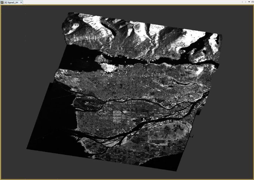
SAR Basics Tutorial

Calibrating the Data
To properly work with the SAR data, the data should first be calibrated. This is especially true when
preparing data for mosaicking where you could have several data products at different incidence angles
and relative levels of brightness.

Radiometric calibration converts backscatter intensity as received by the sensor to the normalized radar
cross section (Sigma0) as a calibrated measure taking into account the global incidence angle of the
image and other sensor-specific characteristics. This makes radar images of different dates, sensors, or
imaging geometries comparable.

The corrections that get applied during calibration are mission-specific, therefore the software will
automatically determine what kind of input product is opened and what corrections need to be applied
based on the product’s metadata. Calibration is essential for quantitative use of SAR data.

Step 2 - Calibrate the product: From the Radar menu, go to Radiometric and select Calibrate.

The source product should be the imported product, the target product will be the new file you will create.
Also select the directory in which the target product will be saved (here: C:\Temp)

                                       Figure 4: Radiometric calibration

If you don’t select any source bands, then the
calibration operator will automatically select all
real and imaginary (i, q) bands. Make sure that
“Save as complex output” is not selected, so that
the calibration operator will produce a single
Sigma0 band per real and imaginary pair.

In case of polarimetric analyses, you select
“Save as complex output”.
Please note that there is a separate tutorial on
polarimetric SAR processing.                                          Figure 5: Calibrated product

                                                                                                           4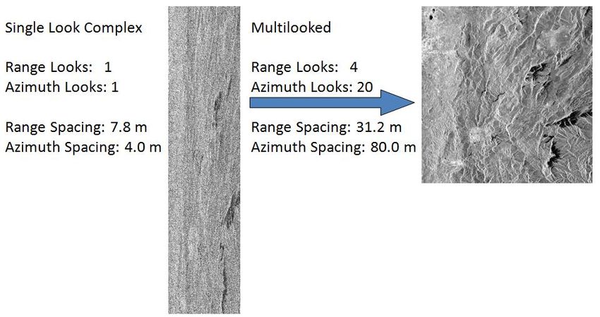
SAR Basics Tutorial

Multilooking
Multilook processing can be used to produce a product with nominal image pixel size.

Multiple looks may be generated by averaging over range and/or azimuth resolution cells improving
radiometric resolution but degrading spatial resolution. As a result, the image will have less noise and
approximate square pixel spacing after being converted from slant range to ground range.

Multilooking can be an optional step since it is not necessary when terrain correcting an image.

Step 3 - Multilook the Intensity_VH band: From the Radar menu, select SAR Utilities and then
Multilooking.

                                    Figure 6: Multilooking an SLC Product

In the Multilook dialog, select the calibrated data as an input and the Sigma0_VH band to only produce
an output for this band (Figure 7).

Specify the number of range looks while the number of azimuth looks is computed based on the ground
range spacing and the azimuth spacing.

Multilooking will produce a ground range square pixel using 1 look in range and 3 looks in azimuth. The
resulting mean ground range pixel size will be 13.95 m.

Press Run to begin processing.

When complete, a new product will be created and will be available in the Products View.

In the new product, open the Sigma0_VH band (Figure 8). The image now looks more proportional;
however, it still contains a lot of noise.

                                                                                                          5
SAR Basics Tutorial

                                 Figure 7: Multilooking of the VH polarization

                      Figure 8: VH polarization before (left) and after multilooking (right)

                                                                                               6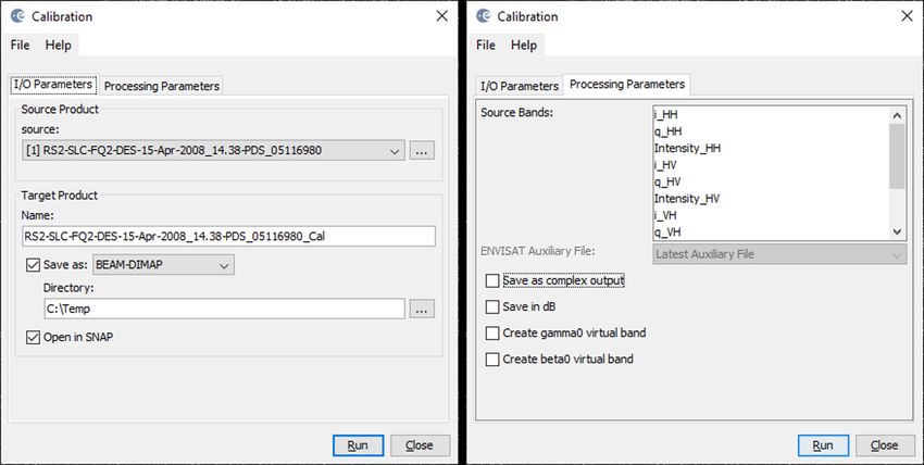
SAR Basics Tutorial

Speckle Reduction
Speckle is caused by random constructive and destructive interference resulting in salt and pepper noise
throughout the image.

Speckle filters can be applied to the data to reduce the amount of speckle at the cost of blurred features
or reduced resolution. Extensive reviews and comparisons of speckle filters are provided by Dong et al.
(2000), Touzi (2002), and Lee et al. (2009). The choice for a best filter often depends on the type of data,
its spatial resolution, the degree of inherent speckle, and the application.

Step 4 - Speckle Filtering: Select the multilooked product and then select Speckle Filtering/Single
Product Speckle Filter from the Radar menu.

From the Speckle Filtering dialog, select the multilooked product as input. In the second tab select the
Refined Lee speckle filter. The Refined Lee filter averages the image while preserving edges. It has no
parameters to set, while others require the definition of a kernel size and other parameters. The effect of
different filters and their parameter configurations has to be explored by careful comparison to find the
best solution for the respective case.

Press Run to process.

                                          Figure 9: Speckle filtering

                                                                                                              7
SAR Basics Tutorial
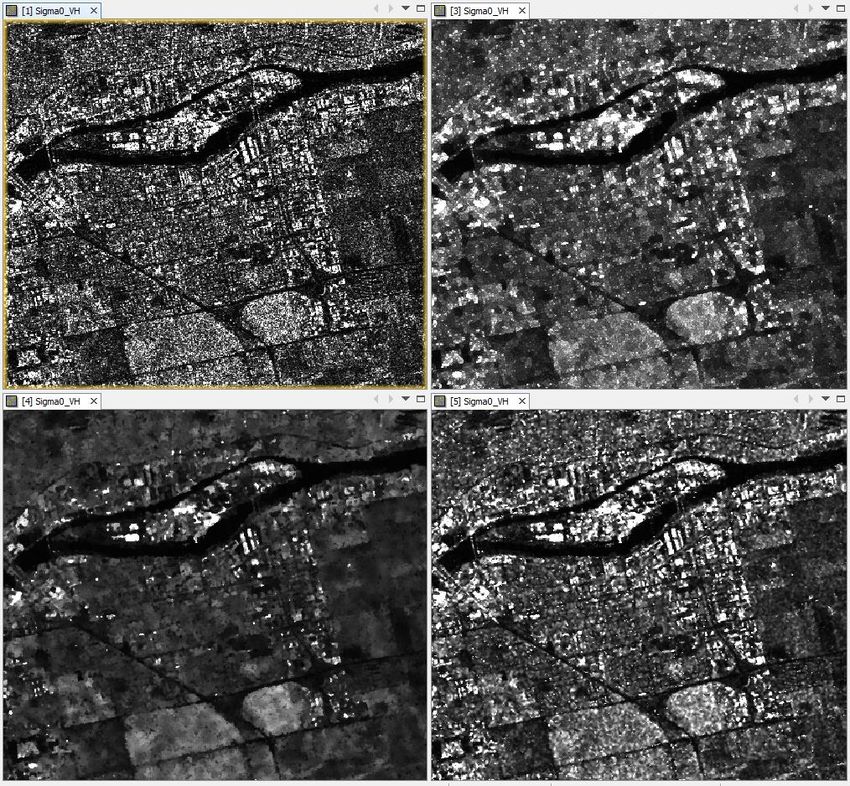
Open the newly created speckle filtered product. You can use the Split Window tools to
compare different products (Figure 10).
Figure 10: Sigma0_VH before speckle filtering (top left),
after Refined Lee filter (top right),
after IDAN filter (bottom left),
and after Frost filter (bottom right)
The final processing which we will perform on this product will be to terrain correction.
8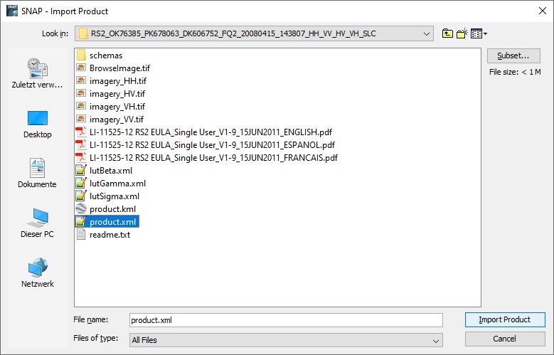
SAR Basics Tutorial
Terrain Correction
Terrain Correction will geocode the image by correcting SAR geometric distortions using a digital
elevation model (DEM) and producing a map projected product.
Geocoding converts an image from slant range or ground range geometry into a map coordinate system.
Terrain geocoding involves using a Digital Elevation Model (DEM) to correct for inherent geometric
distortions, such as foreshortening, layover and shadow (Fehler! Verweisquelle konnte nicht gefunden
werden.). More information on these effects is given in the ESA radar course materials.
Foreshortening
• The period of time a slope is illuminated by the transmitted pulse of the radar energy determines
the length of the slope on radar imagery.
• This results in shortening of a terrain slope on radar imagery in all cases except when the local
angle of incidence () is equal to 90˚.
Layover
• When the top of the terrain slope is closer to the radar platform than the bottom the former will
be recorded sooner than the latter.
• The sequence at which the points along the terrain are imaged produces an image that appears
inverted.
• Radar layover is dependent on the difference in slant range distance between the top and
bottom of the feature.
Shadow
• The back-slope is obscured from the imaging beam causing no return area or radar shadow.
Figure 11: Geometric distortions in radar images (Braun 2019)
9SAR Basics Tutorial
Step 5 - Terrain Correction: Select the speckle filtered product and then select Range-Doppler Terrain
Correction from the SAR Processing/Geometric menu.
By default, the terrain correction will use the SRTM 3Sec DEM (90 m pixel spacing). You can also select a
DEM of higher resolution (SRTM 1Sec HGT (AutoDownlad) 30 m pixel spacing). The software will
automatically determine the DEM tiles needed and download them automatically from internet servers.
The default output map projection is Geographic (based on Latitude/Longitude), but you can also select a
UTM zone.
If you don’t want ocean areas removed (based on the DEM values), disable “Mask areas without
elevation”
Press Run to process.
Figure 12: Range Doppler Terrain Correction
10SAR Basics Tutorial
Open the terrain corrected product. You will see that the terrain correction has worked when the image is
rotated (facing north) and the image boundaries are stretched in mountainous areas (Figure 12).
Terrain Corrected Image
11SAR Basics Tutorial
Conversion to dB scale
As Sigma0 values show the backscatter intensity in linear scale, the majority is dark while only a small
proportion is bright. This is not ideal in a statistical sense and can make image interpretation difficult,
because values of smaller than 1 have similar grey values.
To achieve a normal distribution of values, the log function is applied to the radar image. It translates
the pixel values into a logarithmic scale and yields in higher contrasts, because the bright values are
shifted towards the mean while dark values become stretched over a wider color range (Fehler!
Verweisquelle konnte nicht gefunden werden., bottom).
The value range of calibrated dB data is -35 to +10 dB
Step 5 – Conversion to dB scale: To view the image in decibel scaling, right-click on the terrain
corrected Sigma_VH band and select Linear to/from dB to convert the data using a virtual band (Figure
13 and Figure 14).
Figure 13: Conversion to dB scale
A new virtual band will be created with the expression 10*log10(Intensity_VH). Double-click on the new
Sigma_VH_dB band to open it (Figure 15).
Figure 14: Log-scaled backscatter intensity
12SAR Basics Tutorial
Figure 15: Sigma0 in dB scale
You will see that the values of calibrated dB data roughly range between -35 and +5 dB (Figure 16).
Figure 16: Histogram before (left) and after conversion to dB scale (right)
13SAR Basics Tutorial
For more tutorials visit the Sentinel Toolboxes website
http://step.esa.int/main/doc/tutorials/
Send comments to the SNAP Forum
http://forum.step.esa.int/
14You can also read