SHARPNESS-AWARE MINIMIZATION FOR EFFICIENTLY IMPROVING GENERALIZATION
←
→
Page content transcription
If your browser does not render page correctly, please read the page content below
Under review as a conference paper at ICLR 2021

S HARPNESS -AWARE M INIMIZATION FOR E FFICIENTLY
I MPROVING G ENERALIZATION
 Anonymous authors
 Paper under double-blind review

                                            A BSTRACT

         In today’s heavily overparameterized models, the value of the training loss pro-
         vides few guarantees on model generalization ability. Indeed, optimizing only the
         training loss value, as is commonly done, can easily lead to suboptimal model
         quality. Motivated by prior work connecting the geometry of the loss landscape
         and generalization, we introduce a novel, effective procedure for instead simulta-
         neously minimizing loss value and loss sharpness. In particular, our procedure,
         Sharpness-Aware Minimization (SAM), seeks parameters that lie in neighbor-
         hoods having uniformly low loss; this formulation results in a min-max optimiza-
         tion problem on which gradient descent can be performed efficiently. We present
         empirical results showing that SAM improves model generalization across a va-
         riety of benchmark datasets (e.g., CIFAR-{10, 100}, ImageNet, finetuning tasks)
         and models, yielding novel state-of-the-art performance for several. Additionally,
         we find that SAM natively provides robustness to label noise on par with that
         provided by state-of-the-art procedures that specifically target learning with noisy
         labels.

1   I NTRODUCTION
Modern machine learning’s success in achieving ever better performance on a wide range of tasks
has relied in significant part on ever heavier overparameterization, in conjunction with developing
ever more effective training algorithms that are able to find parameters that generalize well. Indeed,
many modern neural networks can easily memorize the training data and have the capacity to readily
overfit (Zhang et al., 2016). Such heavy overparameterization is currently required to achieve state-
of-the-art results in a variety of domains (Tan & Le, 2019; Kolesnikov et al., 2020; Huang et al.,
2018). In turn, it is essential that such models be trained using procedures that ensure that the
parameters actually selected do in fact generalize beyond the training set.
Unfortunately, simply minimizing commonly used loss functions (e.g., cross-entropy) on the train-
ing set is typically not sufficient to achieve satisfactory generalization. The training loss landscapes
of today’s models are commonly complex and non-convex, with a multiplicity of local and global
minima, and with different global minima yielding models with different generalization abilities
(Shirish Keskar et al., 2016). As a result, the choice of optimizer (and associated optimizer settings)
from among the many available (e.g., stochastic gradient descent (Nesterov, 1983), Adam (Kingma
& Ba, 2014), RMSProp (Hinton et al.), and others (Duchi et al., 2011; Dozat, 2016; Martens &
Grosse, 2015)) has become an important design choice, though understanding of its relationship
to model generalization remains nascent (Shirish Keskar et al., 2016; Wilson et al., 2017; Shirish
Keskar & Socher, 2017; Agarwal et al., 2020; Jacot et al., 2018). Relatedly, a panoply of methods
for modifying the training process have been proposed, including dropout (Srivastava et al., 2014),
batch normalization (Ioffe & Szegedy, 2015), stochastic depth (Huang et al., 2016), data augmenta-
tion (Cubuk et al., 2018), and mixed sample augmentations (Zhang et al., 2017; Harris et al., 2020).
The connection between the geometry of the loss landscape—in particular, the flatness of minima—
and generalization has been studied extensively from both theoretical and empirical perspectives
(Shirish Keskar et al., 2016; Dziugaite & Roy, 2017; Jiang et al., 2019). While this connection
has held the promise of enabling new approaches to model training that yield better generalization,
practical efficient algorithms that specifically seek out flatter minima and furthermore effectively
improve generalization on a range of state-of-the-art models have thus far been elusive (e.g., see

                                                   1
Under review as a conference paper at ICLR 2021
Cifar10
Cifar100
Imagenet
Finetuning
SVHN
F-MNIST
Noisy Cifar
0 20 40
Error reduction (%)
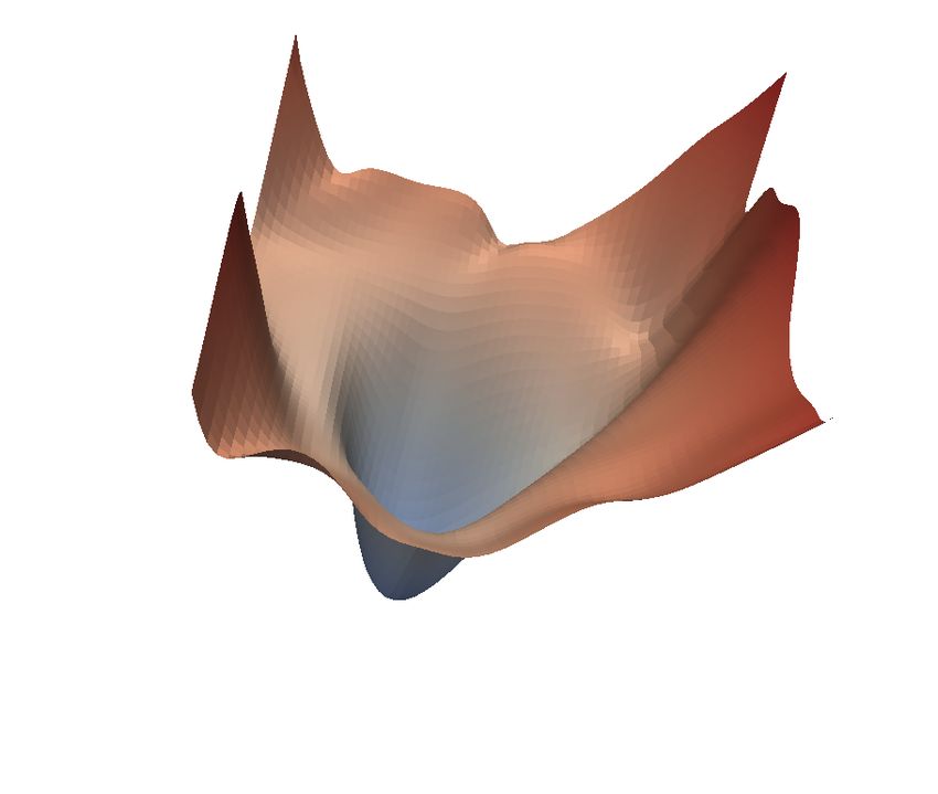
Figure 1: (left) Error rate reduction obtained by switching to SAM. Each point is a different dataset
/ model / data augmentation. (middle) A sharp minimum to which a ResNet trained with SGD
converged. (right) A wide minimum to which the same ResNet trained with SAM converged.
(Chaudhari et al., 2016; Izmailov et al., 2018); we include a more detailed discussion of prior work
in Section 5).
We present here a new efficient, scalable, and effective approach to improving model generalization
ability that directly leverages the geometry of the loss landscape and its connection to generaliza-
tion, and is powerfully complementary to existing techniques. In particular, we make the following
contributions:
• We introduce Sharpness-Aware Minimization (SAM), a novel procedure that improves
model generalization by simultaneously minimizing loss value and loss sharpness. SAM
functions by seeking parameters that lie in neighborhoods having uniformly low loss value
(rather than parameters that only themselves have low loss value, as illustrated in the middle
and righthand images of Figure 1), and can be implemented efficiently and easily.
• We show via a rigorous empirical study that using SAM improves model generalization
ability across a range of widely studied computer vision tasks (e.g., CIFAR-{10, 100},
ImageNet, finetuning tasks) and models, as summarized in the lefthand plot of Figure 1. For
example, applying SAM yields novel state-of-the-art performance for a number of already-
intensely-studied tasks, such as CIFAR-100, SVHN, Fashion-MNIST, and the standard set
of image classification finetuning tasks (e.g., Flowers, Stanford Cars, Oxford Pets, etc).
• We show that SAM furthermore provides robustness to label noise on par with that provided
by state-of-the-art procedures that specifically target learning with noisy labels.
• Through the lens provided by SAM, we further elucidate the connection between loss
sharpness and generalization by surfacing a promising new notion of sharpness, which
we term m-sharpness.
Section 2 below derives the SAM procedure and presents the resulting algorithm in full detail. Sec-
tion 3 evaluates SAM empirically, and Section 4 further analyzes the connection between loss sharp-
ness and generalization through the lens of SAM. Finally, we conclude with an overview of related
work and a discussion of conclusions and future work in Sections 5 and 6, respectively.
2 S HARPNESS -AWARE M INIMIZATION (SAM)
Throughout the paper, we denote scalars as a, vectors as a, matrices as A, sets as A, and equality by
definition as ,. Given a training dataset S , ∪ni=1 {(xi , yi )} drawn i.i.d. from distribution D, we
seek to learn a model that generalizes well. In particular, consider a family of models parameterized
by w ∈ W ⊆ Rd ; given a per-data-point loss function l : W × X × Y → R+ , we define the training
Pn
set loss LS (w) , n1 i=1 l(w, xi , yi ) and the population loss LD (w) , E(x,y)∼D [l(w, x, y)].
Having observed only S, the goal of model training is to select model parameters w having low
population loss LD (w).
Utilizing LS (w) as an estimate of LD (w) motivates the standard approach of selecting parameters
w by solving minw LS (w) (possibly in conjunction with a regularizer on w) using an optimization
2Under review as a conference paper at ICLR 2021
procedure such as SGD or Adam. Unfortunately, however, for modern overparameterized mod-
els such as deep neural networks, typical optimization approaches can easily result in suboptimal
performance at test time. In particular, for modern models, LS (w) is typically non-convex in w,
with multiple local and even global minima that may yield similar values of LS (w) while having
significantly different generalization performance (i.e., significantly different values of LD (w)).
Motivated by the connection between sharpness of the loss landscape and generalization, we propose
a different approach: rather than seeking out parameter values w that simply have low training loss
value LS (w), we seek out parameter values whose entire neighborhoods have uniformly low training
loss value (equivalently, neighborhoods having both low loss and low curvature). The following
theorem illustrates the motivation for this approach by bounding generalization ability in terms of
neighborhood-wise training loss (full theorem statement and proof in Appendix A):
Theorem (stated informally) 1. For any ρ > 0, with high probability over training set S generated
from distribution D,
LD (w) ≤ max LS (w + ) + h(kwk22 /ρ2 ),
kk2 ≤ρ
+ +
where h : R → R is a strictly increasing function (under some technical conditions on LD (w)).
To make explicit our sharpness term, we can rewrite the right hand side of the inequality above as
[ max LS (w + ) − LS (w)] + LS (w) + h(kwk22 /ρ2 ).
kk2 ≤ρ
The term in square brackets captures the sharpness of LS at w by measuring how quickly the training
loss can be increased by moving from w to a nearby parameter value; this sharpness term is then
summed with the training loss value itself and a regularizer on the magnitude of w. Given that
the specific function h is heavily influenced by the details of the proof, we substitute the second
term with λkwk22 /ρ2 for a hyperparameter λ, yielding a standard L2 regularization term. Thus,
inspired by the terms from the bound, we propose to select parameter values by solving the following
Sharpness-Aware Minimization (SAM) problem:
min LSAM
S (w) + λ||w||22 where LSAM
S (w) , max LS (w + ), (1)
w ||||p ≤ρ
where ρ ≥ 0 is a hyperparameter and p ∈ [1, ∞] (we have generalized slightly from an L2-norm
to a p-norm in the maximization over , though we show empirically in appendix C.5 that p = 2 is
typically optimal). Figure 1 shows1 the loss landscape for a model that converged to minima found
by minimizing either LS (w) or LSAM
S (w), illustrating that the sharpness-aware loss prevents the
model from converging to a sharp minimum.
In order to minimize LSAM S (w), we derive an efficient and effective approximation to
∇w LSAM
S (w) by differentiating through the inner maximization, which in turn enables us to apply
stochastic gradient descent directly to the SAM objective. Proceeding down this path, we first ap-
proximate the inner maximization problem via a first-order Taylor expansion of LS (w + ) w.r.t.
around 0, obtaining
∗ (w) , arg max LS (w + ) ≈ arg max LS (w) + T ∇w LS (w) = arg max T ∇w LS (w).
kkp ≤ρ kkp ≤ρ kkp ≤ρ
In turn, the value ˆ(w) that solves this approximation is given by the solution to a classical dual
norm problem (| · |q−1 denotes elementwise absolute value and power) 2 :
1/p
q−1
ˆ(w) = ρ sign (∇w LS (w)) |∇w LS (w)| / k∇w LS (w)kqq (2)
where 1/p + 1/q = 1. Substituting back into equation (1) and differentiating, we then have
d(w + ˆ(w))
∇w LSAM
S (w) ≈ ∇w LS (w + ˆ(w)) = ∇w LS (w)|w+ˆ(w)
dw
dˆ
(w)
= ∇w LS (w)|w+ˆ(w) + ∇w LS (w)|w+ˆ(w) .
dw
1
Figure 1 was generated following Li et al. (2017) with the provided ResNet56 (no residual connections)
checkpoint, and training the same model with SAM.
2
In the case of interest p = 2, this boils down to simply rescaling the gradient such that its norm is ρ.
3Under review as a conference paper at ICLR 2021
This approximation to ∇w LSAMS (w) can be straightforwardly computed via automatic differentia-
tion, as implemented in common libraries such as JAX, TensorFlow, and PyTorch. Though this com-
putation implicitly depends on the Hessian of LS (w) because ˆ(w) is itself a function of ∇w LS (w),
the Hessian enters only via Hessian-vector products, which can be computed tractably without ma-
terializing the Hessian matrix. Nonetheless, to further accelerate the computation, we drop the
second-order terms. obtaining our final gradient approximation:
∇w LSAM
S (w) ≈ ∇w LS (w)|w+ˆ(w) . (3)
As shown by the results in Section 3, this approximation (without the second-order terms) yields an
effective algorithm. In Appendix C.4, we additionally investigate the effect of instead including the
second-order terms; in that initial experiment, including them surprisingly degrades performance,
and further investigating these terms’ effect should be a priority in future work.
We obtain the final SAM algorithm by applying a standard numerical optimizer such as stochastic
gradient descent (SGD) to the SAM objective LSAMS (w), using equation 3 to compute the requisite
objective function gradients. Algorithm 1 gives pseudo-code for the full SAM algorithm, using SGD
as the base optimizer, and Figure 2 schematically illustrates a single SAM parameter update.
Input: Training set S , ∪n i=1 {(xi , yi )}, Loss function
l : W × X × Y → R+ , Batch size b, Step size η > 0,
Neighborhood size ρ > 0.
L(wt) wt + 1
Output: Model trained with SAM
Initialize weights w0 , t = 0;
while not converged do L(wt) wt wtSAM
+1
Sample batch B = {(x1 , y1 ), ...(xb , yb )}; || L(wt)||2
Compute gradient ∇w LB (w) of the batch’s training loss;
Compute ˆ(w) per equation 2; wadv L(wadv)
Compute gradient approximation for the SAM objective
(equation 3): g = ∇w LB (w)|w+ˆ(w) ;
Update weights: wt+1 = wt − ηg;
t = t + 1;
end Figure 2: Schematic of the SAM param-
return wt eter update.
Algorithm 1: SAM algorithm
3 E MPIRICAL E VALUATION
In order to assess SAM’s efficacy, we apply it to a range of different tasks, including image clas-
sification from scratch (including on CIFAR-10, CIFAR-100, and ImageNet), finetuning pretrained
models, and learning with noisy labels. In all cases, we measure the benefit of using SAM by simply
replacing the optimization procedure used to train existing models with SAM, and computing the
resulting effect on model generalization. As seen below, SAM materially improves generalization
performance in the vast majority of these cases.
3.1 I MAGE C LASSIFICATION F ROM S CRATCH
We first evaluate SAM’s impact on generalization for today’s state-of-the-art models on CIFAR-10
and CIFAR-100 (without pretraining): WideResNets with ShakeShake regularization (Zagoruyko
& Komodakis, 2016; Gastaldi, 2017) and PyramidNet with ShakeDrop regularization (Han et al.,
2016; Yamada et al., 2018). Note that some of these models have already been heavily tuned in
prior work and include carefully chosen regularization schemes to prevent overfitting; therefore,
significantly improving their generalization is quite non-trivial. We have ensured that our imple-
mentations’ generalization performance in the absence of SAM matches or exceeds that reported in
prior work (Cubuk et al., 2018; Lim et al., 2019)
All results use basic data augmentations (horizontal flip, padding by four pixels, and random crop).
We also evaluate in the setting of more advanced data augmentation methods such as cutout regu-
larization (Devries & Taylor, 2017) and AutoAugment (Cubuk et al., 2018), which are utilized by
prior work to achieve state-of-the-art results.
4Under review as a conference paper at ICLR 2021
SAM has a single hyperparameter ρ (the neighborhood size), which we tune via a grid search over
{0.01, 0.02, 0.05, 0.1, 0.2, 0.5} using 10% of the training set as a validation set. Please see ap-
pendix C.1 for the values of all hyperparameters and additional training details. As each SAM
weight update requires two backpropagation operations (one to compute ˆ(w) and another to com-
pute the final gradient), we allow each non-SAM training run to execute twice as many epochs as
each SAM training run, and we report the best score achieved by each non-SAM training run across
either the standard epoch count or the doubled epoch count 3 . We run five independent replicas of
each experimental condition for which we report results (each with independent weight initialization
and data shuffling), reporting the resulting mean error (or accuracy) on the test set, and the associ-
ated 95% confidence interval. Our implementations utilize JAX (Bradbury et al., 2018), and we
train all models on a single host having 8 Nvidia V100 GPUs. To compute the SAM update when
parallelizing across multiple accelerators, we divide each data batch evenly among the accelerators,
independently compute the SAM gradient on each accelerator, and average the resulting sub-batch
SAM gradients to obtain the final SAM update.
As seen in Table 1, SAM improves generalization across all settings evaluated for CIFAR-10 and
CIFAR-100. For example, SAM enables a simple WideResNet to attain 1.6% test error, versus
2.2% error without SAM. Such gains have previously been attainable only by using more complex
model architectures (e.g., PyramidNet) and regularization schemes (e.g., Shake-Shake, ShakeDrop);
SAM provides an easily-implemented, model-independent alternative. Furthermore, SAM delivers
improvements even when applied atop complex architectures that already use sophisticated regular-
ization: for instance, applying SAM to a PyramidNet with ShakeDrop regularization yields 10.3%
error on CIFAR-100, which is, to our knowledge, a new state of the art on this dataset without the
use of additional data.
CIFAR-10 CIFAR-100
Model Augmentation SAM SGD SAM SGD
WRN-28-10 (200 epochs) Basic 2.7±0.1 3.5±0.1 16.5±0.2 18.8±0.2
WRN-28-10 (200 epochs) Cutout 2.3±0.1 2.6±0.1 14.9±0.2 16.9±0.1
WRN-28-10 (200 epochs) AA 2.1±Under review as a conference paper at ICLR 2021
As seen in Table 2, SAM again consistently improves performance, for example improving the
ImageNet top-1 error rate of ResNet-152 from 20.3% to 18.4%. Furthermore, note that SAM enables
increasing the number of training epochs while continuing to improve accuracy without overfitting.
In contrast, the standard training procedure (without SAM) generally significantly overfits as training
extends from 200 to 400 epochs.
SAM Standard Training (No SAM)
Model Epoch
Top-1 Top-5 Top-1 Top-5
ResNet-50 100 22.5±0.1 6.28±0.08 22.9±0.1 6.62±0.11
200 21.4±0.1 5.82±0.03 22.3±0.1 6.37±0.04
400 20.9±0.1 5.51±0.03 22.3±0.1 6.40±0.06
ResNet-101 100 20.2±0.1 5.12±0.03 21.2±0.1 5.66±0.05
200 19.4±0.1 4.76±0.03 20.9±0.1 5.66±0.04
400 19.0±Under review as a conference paper at ICLR 2021
3.3 ROBUSTNESS TO L ABEL N OISE
The fact that SAM seeks out model parameters that
are robust to perturbations suggests SAM’s poten- Method Noise rate (%)
tial to provide robustness to noise in the training set 20 40 60 80
(which would perturb the training loss landscape). Sanchez et al. (2019) 94.0 92.8 90.3 74.1
Zhang & Sabuncu (2018) 89.7 87.6 82.7 67.9
Thus, we assess here the degree of robustness that Lee et al. (2019) 87.1 81.8 75.4 -
SAM provides to label noise. Chen et al. (2019) 89.7 - - 52.3
Huang et al. (2019) 92.6 90.3 43.4 -
In particular, we measure the effect of apply- MentorNet (2017) 92.0 91.2 74.2 60.0
ing SAM in the classical noisy-label setting for Mixup (2017) 94.0 91.5 86.8 76.9
CIFAR-10, in which a fraction of the training set’s MentorMix (2019) 95.6 94.2 91.3 81.0
SGD 84.8 68.8 48.2 26.2
labels are randomly flipped; the test set remains Mixup 93.0 90.0 83.8 70.2
unmodified (i.e., clean). To ensure valid compar- Bootstrap + Mixup 93.3 92.0 87.6 72.0
ison to prior work, which often utilizes architec- SAM 95.1 93.4 90.5 77.9
tures specialized to the noisy-label setting, we train Bootstrap + SAM 95.4 94.2 91.8 79.9
a simple model of similar size (ResNet-32) for 200
epochs, following Jiang et al. (2019). We evalu- Table 4: Test accuracy on the clean test set
ate five variants of model training: standard SGD, for models trained on CIFAR-10 with noisy la-
SGD with Mixup (Zhang et al., 2017), SAM, and bels. Lower block is our implementation, up-
”bootstrapped” variants of SGD with Mixup and per block gives scores from the literature, per
SAM (wherein the model is first trained as usual Jiang et al. (2019).
and then retrained from scratch on the labels pre-
dicted by the initially trained model). When apply-
ing SAM, we use ρ = 0.1 for all noise levels except 80%, for which we use ρ = 0.05 for more stable
convergence. For the Mixup baselines, we tried all values of α ∈ {1, 8, 16, 32} and conservatively
report the best score for each noise level.
As seen in Table 4, SAM provides a high degree of robustness to label noise, on par with that
provided by state-of-the art procedures that specifically target learning with noisy labels. Indeed,
simply training a model with SAM outperforms all prior methods specifically targeting label noise
robustness, with the exception of MentorMix (Jiang et al., 2019). However, simply bootstrapping
SAM yields performance comparable to that of MentorMix (which is substantially more complex).
4 S HARPNESS AND G ENERALIZATION T HROUGH THE L ENS OF SAM
4.1 m- SHARPNESS
Though our derivation of SAM defines the SAM objective over the entire training set, when utilizing
SAM in practice, we compute the SAM update per-batch (as described in Algorithm 1) or even by
averaging SAM updates computed independently per-accelerator (where each accelerator receives a
subset of size m of a batch, as described in Section 3). This latter setting is equivalent to modifying
the SAM objective (equation 1) to sum over a set of independent maximizations, each performed
on a sum of per-data-point losses on a disjoint subset of m data points, rather than performing the
maximization over a global sum over the training set (which would be equivalent to setting m
to the total training set size). We term the associated measure of sharpness of the loss landscape
m-sharpness.
To better understand the effect of m on SAM, we train a small ResNet on CIFAR-10 using SAM
with a range of values of m. As seen in Figure 3 (middle), smaller values of m tend to yield models
having better generalization ability. This relationship fortuitously aligns with the need to parallelize
across multiple accelerators in order to scale training for many of today’s models.
Intriguingly, the m-sharpness measure described above furthermore exhibits better correlation with
models’ actual generalization gaps as m decreases, as demonstrated by Figure 3 (right)5 . In partic-
ular, this implies that m-sharpness with m < n yields a better predictor of generalization than the
5
We follow the rigorous framework of Jiang et al. (2019), reporting the mutual information between
the m-sharpness measure and generalization on the two publicly available tasks from the Predicting gen-
eralization in deep learning NeurIPS2020 competition. https://competitions.codalab.org/
competitions/25301
7Under review as a conference paper at ICLR 2021
SGD SAM
max = 62.9 max = 18.6
Epoch: 1
max/ 5 = 2.5 max/ 5 = 3.6 0.08 0.050
m Task 1
0 20 40 60 0 20 40 60 1 0.045 Task 2 0.17
Mutual information
Mutual information
0.07 4
Error rate (%)
max = 12.5 max = 8.9 16
Epoch: 50
max/ 5 = 1.7 max/ 5 = 1.9 64 0.040 0.16
0.06 256
0 5 10 0 5 10
0.035 0.15
0.05
max = 24.2 max = 1.0 0.030
Epoch: 300
0.14
max/ 5 = 11.4 max/ 5 = 2.6
0.04
0 10 20 0 10 20
0.00 0.05 0.10 0.15 1 4 16 64 256
p( ) p( ) m
Figure 3: (left) Evolution of the spectrum of the Hessian during training of a model with standard
SGD (lefthand column) or SAM (righthand column). (middle) Test error as a function of ρ for dif-
ferent values of m. (right) Predictive power of m-sharpness for the generalization gap, for different
values of m (higher means the sharpness measure is more correlated with actual generalization gap).
full-training-set measure suggested by Theorem 1 in Section 2 above, suggesting an interesting new
avenue of future work for understanding generalization.
4.2 H ESSIAN S PECTRA
Motivated by the connection between geometry of the loss landscape and generalization, we con-
structed SAM to seek out minima of the training loss landscape having both low loss value and low
curvature (i.e., low sharpness). To further confirm that SAM does in fact find minima having low
curvature, we compute the spectrum of the Hessian for a WideResNet40-10 trained on CIFAR-10
for 300 steps both with and without SAM (without batch norm, which tends to obscure interpretation
of the Hessian), at different epochs during training. Due to the parameter space’s dimensionality, we
approximate the Hessian spectrum using the Lanczos algorithm of Ghorbani et al. (2019).
Figure 3 (left) reports the resulting Hessian spectra. As expected, the models trained with SAM
converge to minima having lower curvature, as seen in the overall distribution of eigenvalues, the
maximum eigenvalue (λmax ) at convergence (approximately 25 without SAM, 1.0 with SAM), and
the bulk of the spectrum (the ratio λmax /λ5 , commonly used as a proxy for sharpness (Jastrzebski
et al., 2020); up to 11.4 without SAM, and 2.6 with SAM).
5 R ELATED W ORK
The idea of searching for “flat” minima can be traced back to Hochreiter & Schmidhuber (1995), and
its connection to generalization has seen significant study (Shirish Keskar et al., 2016; Dziugaite &
Roy, 2017; Neyshabur et al., 2017; Dinh et al., 2017). In a recent large scale empirical study, Jiang
et al. (2019) studied 40 complexity measures and showed that a sharpness-based measure has highest
correlation with generalization, which motivates penalizing sharpness. Hochreiter & Schmidhuber
(1997) was perhaps the first paper on penalizing the sharpness, regularizing a notion related to Min-
imum Description Length (MDL). Other ideas which also penalize sharp minima include operating
on diffused loss landscape (Mobahi, 2016) and regularizing local entropy (Chaudhari et al., 2016).
Another direction is to not penalize the sharpness explicitly, but rather average weights during train-
ing; Izmailov et al. (2018) showed that doing so can yield flatter minima that can also generalize
better. However, the measures of sharpness proposed previously are difficult to compute and differ-
entiate through. In contrast, SAM is highly scalable as it only needs one gradient computation. The
concurrent work of Sun et al. (2020) focuses on resilience to random and adversarial corruption to
expose a model’s vulnerabilities; this work is perhaps closest to ours. Our work has a different ba-
sis: we develop SAM motivated by a principled starting point in generalization, clearly demonstrate
SAM’s efficacy via rigorous large-scale empirical evaluation, and surface important practical and
theoretical facets of the procedure (e.g., m-sharpness). The notion of all-layer margin introduced by
Wei & Ma (2020) is closely related to this work; one is adversarial perturbation over the activations
of a network and the other over its weights, and there is some coupling between these two quantities.
8Under review as a conference paper at ICLR 2021
6 D ISCUSSION AND F UTURE W ORK
In this work, we have introduced SAM, a novel algorithm that improves generalization by simulta-
neously minimizing loss value and loss sharpness; we have demonstrated SAM’s efficacy through a
rigorous large-scale empirical evaluation. We have surfaced a number of interesting avenues for fu-
ture work. On the theoretical side, the notion of per-data-point sharpness yielded by m-sharpness (in
contrast to global sharpness computed over the entire training set, as has typically been studied in the
past) suggests an interesting new lens through which to study generalization. Methodologically, our
results suggest that SAM could potentially be used in place of Mixup in robust or semi-supervised
methods that currently rely on Mixup (giving, for instance, MentorSAM). We leave to future work
a more in-depth investigation of these possibilities.
R EFERENCES
Naman Agarwal, Rohan Anil, Elad Hazan, Tomer Koren, and Cyril Zhang. Revisiting the gener-
alization of adaptive gradient methods, 2020. URL https://openreview.net/forum?
id=BJl6t64tvr.
James Bradbury, Roy Frostig, Peter Hawkins, Matthew James Johnson, Chris Leary, Dougal
Maclaurin, and Skye Wanderman-Milne. JAX: composable transformations of Python+NumPy
programs, 2018. URL http://github.com/google/jax.
Niladri S Chatterji, Behnam Neyshabur, and Hanie Sedghi. The intriguing role of module criticality
in the generalization of deep networks. In International Conference on Learning Representations,
2020.
Pratik Chaudhari, Anna Choromanska, Stefano Soatto, Yann LeCun, Carlo Baldassi, Christian
Borgs, Jennifer Chayes, Levent Sagun, and Riccardo Zecchina. Entropy-SGD: Biasing Gradi-
ent Descent Into Wide Valleys. arXiv e-prints, art. arXiv:1611.01838, November 2016.
Pengfei Chen, Benben Liao, Guangyong Chen, and Shengyu Zhang. Understanding and utilizing
deep neural networks trained with noisy labels. CoRR, abs/1905.05040, 2019. URL http:
//arxiv.org/abs/1905.05040.
Ekin Dogus Cubuk, Barret Zoph, Dandelion Mané, Vijay Vasudevan, and Quoc V. Le. Au-
toaugment: Learning augmentation policies from data. CoRR, abs/1805.09501, 2018. URL
http://arxiv.org/abs/1805.09501.
J. Deng, W. Dong, R. Socher, L.-J. Li, K. Li, and L. Fei-Fei. ImageNet: A Large-Scale Hierarchical
Image Database. In CVPR09, 2009.
Terrance Devries and Graham W. Taylor. Improved regularization of convolutional neural networks
with cutout. CoRR, abs/1708.04552, 2017. URL http://arxiv.org/abs/1708.04552.
Laurent Dinh, Razvan Pascanu, Samy Bengio, and Yoshua Bengio. Sharp minima can generalize
for deep nets. arXiv preprint arXiv:1703.04933, 2017.
Alexey Dosovitskiy, Lucas Beyer, Alexander Kolesnikov, Dirk Weissenborn, Xiaohua Zhai, Thomas
Unterthiner, Mostafa Dehghani, Matthias Minderer, Georg Heigold, Sylvain Gelly, Jakob Uszko-
reit, and Neil Houlsby. An Image is Worth 16x16 Words: Transformers for Image Recognition at
Scale. arXiv e-prints, art. arXiv:2010.11929, October 2020.
Timothy Dozat. Incorporating nesterov momentum into adam. 2016.
John Duchi, Elad Hazan, and Yoram Singer. Adaptive subgradient methods for online learning and
stochastic optimization. Journal of machine learning research, 12(7), 2011.
Gintare Karolina Dziugaite and Daniel M Roy. Computing nonvacuous generalization bounds for
deep (stochastic) neural networks with many more parameters than training data. arXiv preprint
arXiv:1703.11008, 2017.
Xavier Gastaldi. Shake-shake regularization. CoRR, abs/1705.07485, 2017. URL http:
//arxiv.org/abs/1705.07485.
9Under review as a conference paper at ICLR 2021
Behrooz Ghorbani, Shankar Krishnan, and Ying Xiao. An Investigation into Neural Net Optimiza-
tion via Hessian Eigenvalue Density. arXiv e-prints, art. arXiv:1901.10159, January 2019.
Dongyoon Han, Jiwhan Kim, and Junmo Kim. Deep pyramidal residual networks. CoRR,
abs/1610.02915, 2016. URL http://arxiv.org/abs/1610.02915.
Ethan Harris, Antonia Marcu, Matthew Painter, Mahesan Niranjan, Adam Prügel-Bennett, and
Jonathon Hare. FMix: Enhancing Mixed Sample Data Augmentation. arXiv e-prints, art.
arXiv:2002.12047, February 2020.
Kaiming He, Xiangyu Zhang, Shaoqing Ren, and Jian Sun. Deep residual learning for image recog-
nition. CoRR, abs/1512.03385, 2015. URL http://arxiv.org/abs/1512.03385.
Geoffrey Hinton, Nitish Srivastava, and Kevin Swersky. Neural networks for machine learning
lecture 6a overview of mini-batch gradient descent.
Sepp Hochreiter and Jürgen Schmidhuber. Simplifying neural nets by discovering flat minima. In
Advances in neural information processing systems, pp. 529–536, 1995.
Sepp Hochreiter and Jürgen Schmidhuber. Flat minima. Neural Computation, 9(1):1–42, 1997.
Gao Huang, Yu Sun, Zhuang Liu, Daniel Sedra, and Kilian Weinberger. Deep Networks with
Stochastic Depth. arXiv e-prints, art. arXiv:1603.09382, March 2016.
J. Huang, L. Qu, R. Jia, and B. Zhao. O2u-net: A simple noisy label detection approach for deep
neural networks. In 2019 IEEE/CVF International Conference on Computer Vision (ICCV), pp.
3325–3333, 2019.
Yanping Huang, Youlong Cheng, Ankur Bapna, Orhan Firat, Mia Xu Chen, Dehao Chen, Hy-
oukJoong Lee, Jiquan Ngiam, Quoc V. Le, Yonghui Wu, and Zhifeng Chen. GPipe: Ef-
ficient Training of Giant Neural Networks using Pipeline Parallelism. arXiv e-prints, art.
arXiv:1811.06965, November 2018.
Sergey Ioffe and Christian Szegedy. Batch normalization: Accelerating deep network training by
reducing internal covariate shift. arXiv preprint arXiv:1502.03167, 2015.
Pavel Izmailov, Dmitrii Podoprikhin, Timur Garipov, Dmitry Vetrov, and Andrew Gordon Wil-
son. Averaging Weights Leads to Wider Optima and Better Generalization. arXiv e-prints, art.
arXiv:1803.05407, March 2018.
Arthur Jacot, Franck Gabriel, and Clément Hongler. Neural tangent kernel: Convergence and gener-
alization in neural networks. CoRR, abs/1806.07572, 2018. URL http://arxiv.org/abs/
1806.07572.
Stanislaw Jastrzebski, Maciej Szymczak, Stanislav Fort, Devansh Arpit, Jacek Tabor, Kyunghyun
Cho, and Krzysztof Geras. The Break-Even Point on Optimization Trajectories of Deep Neural
Networks. arXiv e-prints, art. arXiv:2002.09572, February 2020.
Lu Jiang, Zhengyuan Zhou, Thomas Leung, Li-Jia Li, and Li Fei-Fei. Mentornet: Regularizing
very deep neural networks on corrupted labels. CoRR, abs/1712.05055, 2017. URL http:
//arxiv.org/abs/1712.05055.
Lu Jiang, Di Huang, Mason Liu, and Weilong Yang. Beyond Synthetic Noise: Deep Learning on
Controlled Noisy Labels. arXiv e-prints, art. arXiv:1911.09781, November 2019.
Yiding Jiang, Behnam Neyshabur, Hossein Mobahi, Dilip Krishnan, and Samy Bengio. Fantastic
generalization measures and where to find them. arXiv preprint arXiv:1912.02178, 2019.
Diederik P. Kingma and Jimmy Ba. Adam: A Method for Stochastic Optimization. arXiv e-prints,
art. arXiv:1412.6980, December 2014.
Alexander Kolesnikov, Lucas Beyer, Xiaohua Zhai, Joan Puigcerver, Jessica Yung, Sylvain Gelly,
and Neil Houlsby. Big transfer (bit): General visual representation learning, 2020.
10Under review as a conference paper at ICLR 2021
Simon Kornblith, Jonathon Shlens, and Quoc V. Le. Do Better ImageNet Models Transfer Better?
arXiv e-prints, art. arXiv:1805.08974, May 2018.
John Langford and Rich Caruana. (not) bounding the true error. In Advances in Neural Information
Processing Systems, pp. 809–816, 2002.
Beatrice Laurent and Pascal Massart. Adaptive estimation of a quadratic functional by model selec-
tion. Annals of Statistics, pp. 1302–1338, 2000.
Kimin Lee, Sukmin Yun, Kibok Lee, Honglak Lee, Bo Li, and Jinwoo Shin. Robust inference via
generative classifiers for handling noisy labels, 2019.
Hao Li, Zheng Xu, Gavin Taylor, and Tom Goldstein. Visualizing the loss landscape of neural nets.
CoRR, abs/1712.09913, 2017. URL http://arxiv.org/abs/1712.09913.
Sungbin Lim, Ildoo Kim, Taesup Kim, Chiheon Kim, and Sungwoong Kim. Fast autoaugment.
CoRR, abs/1905.00397, 2019. URL http://arxiv.org/abs/1905.00397.
James Martens and Roger Grosse. Optimizing Neural Networks with Kronecker-factored Approxi-
mate Curvature. arXiv e-prints, art. arXiv:1503.05671, March 2015.
David A McAllester. Pac-bayesian model averaging. In Proceedings of the twelfth annual confer-
ence on Computational learning theory, pp. 164–170, 1999.
Hossein Mobahi. Training recurrent neural networks by diffusion. CoRR, abs/1601.04114, 2016.
URL http://arxiv.org/abs/1601.04114.
Y. E. Nesterov. A method for solving the convex programming problem with convergence rate
o(1/k 2 ). Dokl. Akad. Nauk SSSR, 269:543–547, 1983. URL https://ci.nii.ac.jp/
naid/10029946121/en/.
Yuval Netzer, Tao Wang, Adam Coates, Alessandro Bissacco, Bo Wu, and Andrew Y Ng. Reading
digits in natural images with unsupervised feature learning. 2011.
Behnam Neyshabur, Srinadh Bhojanapalli, David McAllester, and Nati Srebro. Exploring general-
ization in deep learning. In Advances in neural information processing systems, pp. 5947–5956,
2017.
Jiquan Ngiam, Daiyi Peng, Vijay Vasudevan, Simon Kornblith, Quoc V. Le, and Ruoming Pang.
Domain adaptive transfer learning with specialist models. CoRR, abs/1811.07056, 2018. URL
http://arxiv.org/abs/1811.07056.
Eric Arazo Sanchez, Diego Ortego, Paul Albert, Noel E. O’Connor, and Kevin McGuinness. Un-
supervised label noise modeling and loss correction. CoRR, abs/1904.11238, 2019. URL
http://arxiv.org/abs/1904.11238.
Nitish Shirish Keskar and Richard Socher. Improving Generalization Performance by Switching
from Adam to SGD. arXiv e-prints, art. arXiv:1712.07628, December 2017.
Nitish Shirish Keskar, Dheevatsa Mudigere, Jorge Nocedal, Mikhail Smelyanskiy, and Ping Tak Pe-
ter Tang. On Large-Batch Training for Deep Learning: Generalization Gap and Sharp Minima.
arXiv e-prints, art. arXiv:1609.04836, September 2016.
Nitish Srivastava, Geoffrey Hinton, Alex Krizhevsky, Ilya Sutskever, and Ruslan Salakhutdinov.
Dropout: a simple way to prevent neural networks from overfitting. The journal of machine
learning research, 15(1):1929–1958, 2014.
Xu Sun, Zhiyuan Zhang, Xuancheng Ren, Ruixuan Luo, and Liangyou Li. Exploring the Vul-
nerability of Deep Neural Networks: A Study of Parameter Corruption. arXiv e-prints, art.
arXiv:2006.05620, June 2020.
Christian Szegedy, Vincent Vanhoucke, Sergey Ioffe, Jonathon Shlens, and Zbigniew Wojna. Re-
thinking the inception architecture for computer vision, 2015.
11Under review as a conference paper at ICLR 2021
Mingxing Tan and Quoc V. Le. EfficientNet: Rethinking Model Scaling for Convolutional Neural
Networks. arXiv e-prints, art. arXiv:1905.11946, May 2019.
Colin Wei and Tengyu Ma. Improved sample complexities for deep neural networks and robust
classification via an all-layer margin. In International Conference on Learning Representations,
2020.
Longhui Wei, An Xiao, Lingxi Xie, Xin Chen, Xiaopeng Zhang, and Qi Tian. Circumventing
Outliers of AutoAugment with Knowledge Distillation. arXiv e-prints, art. arXiv:2003.11342,
March 2020.
Ashia C Wilson, Rebecca Roelofs, Mitchell Stern, Nati Srebro, and Benjamin Recht. The marginal
value of adaptive gradient methods in machine learning. In Advances in neural information pro-
cessing systems, pp. 4148–4158, 2017.
Han Xiao, Kashif Rasul, and Roland Vollgraf. Fashion-mnist: a novel image dataset for benchmark-
ing machine learning algorithms. CoRR, abs/1708.07747, 2017. URL http://arxiv.org/
abs/1708.07747.
Yoshihiro Yamada, Masakazu Iwamura, and Koichi Kise. Shakedrop regularization. CoRR,
abs/1802.02375, 2018. URL http://arxiv.org/abs/1802.02375.
Sergey Zagoruyko and Nikos Komodakis. Wide residual networks. CoRR, abs/1605.07146, 2016.
URL http://arxiv.org/abs/1605.07146.
Chiyuan Zhang, Samy Bengio, Moritz Hardt, Benjamin Recht, and Oriol Vinyals. Understanding
deep learning requires rethinking generalization. CoRR, abs/1611.03530, 2016. URL http:
//arxiv.org/abs/1611.03530.
Fan Zhang, Meng Li, Guisheng Zhai, and Yizhao Liu. Multi-branch and multi-scale attention learn-
ing for fine-grained visual categorization, 2020.
Hongyi Zhang, Moustapha Cisse, Yann N Dauphin, and David Lopez-Paz. mixup: Beyond empirical
risk minimization. arXiv preprint arXiv:1710.09412, 2017.
Zhilu Zhang and Mert R. Sabuncu. Generalized cross entropy loss for training deep neural networks
with noisy labels. CoRR, abs/1805.07836, 2018. URL http://arxiv.org/abs/1805.
07836.
A A PPENDIX
A.1 PAC BAYESIAN G ENERALIZATION B OUND
Below, we state a generalization bound based on sharpness.
Theorem 2. For any ρ > 0 and any distribution D, with probability 1 − δ over the choice of the
training set S ∼ D,
v
u q 2 !
u k log 1 + kwk22 1 + log(n)
u
u ρ2 k + 4 log nδ + Õ(1)
t
LD (w) ≤ max LS (w + ) + (4)
kk2 ≤ρ n−1
where n = |S|, k is the number of parameters and we assumed LD (w) ≤ Ei ∼N (0,ρ) [LD (w + )].
The condition LD (w) ≤ Ei ∼N (0,ρ) [LD (w + )] means that adding Gaussian perturbation should
not decrease the test error. This is expected to hold in practice for the final solution but does not
necessarily hold for any w.
12Under review as a conference paper at ICLR 2021
p First, note that the right hand side of the bound in the theorem statement is lower bounded
Proof.
by k log(1 + kwk22 /ρ2 )/(4n) which is greater than 1 when kwk22 > ρ2 (exp(4n/k) − 1). In
that case, the right hand side becomes greater than 1 in which case the inequality holds trivially.
Therefore, in the rest of the proof, we only consider the case when kwk22 ≤ ρ2 (exp(4n/k) − 1).
The proof technique we use here is inspired from Chatterji et al. (2020). Using PAC-Bayesian
generalization bound McAllester (1999) and following Dziugaite & Roy (2017), the following gen-
eralization bound holds for any prior P over parameters with probability 1 − δ over the choice of
the training set S, for any posterior Q over parameters:
s
KL(Q||P) + log nδ
Ew∼Q [LD (w)] ≤ Ew∼Q [LS (w)] + (5)
2(n − 1)
Moreover, if P = N (µP , σP2 I) and Q = N (µQ , σQ
2
I), then the KL divergence can be written as
follows:
2 !
1 kσQ + kµP − µQ k22 σP2
KL(P||Q) = − k + k log (6)
2 σP2 σQ2
Given a posterior standard deviation σQ , one could choose a prior standard deviation σP to minimize
the above KL divergence and hence the generalization bound by taking the derivative6 of the above
KL with respect to σP and setting it to zero. We would then have σP∗ 2 = σQ 2
+ kµP − µQ k22 /k.
However, since σP should be chosen before observing the training data S and µQ ,σQ could depend
on S, we are not allowed to optimize σP in this way. Instead, one can have a set of predefined
values for σP and pick the best one in that set. See Langford & Caruana (2002) for the discussion
around this technique. Given fixed a, b > 0, let T = {c exp((1 − j)/k)|j ∈ N} be that predefined
set of values for σP2 . If for any j ∈ N, the above PAC-Bayesian bound holds for σP2 = c exp((1 −
j)/k) with probability 1 − δj with δj = π6δ 2 2 , then by the union bound, all above bounds hold
Pj ∞ 6δ
simultaneously with probability at least 1 − j=1 π2 j 2 = 1 − δ.
Let σQ = ρ, µQ = w and µP = 0. Therefore, we have:
2
σQ + kµP − µQ k22 /k ≤ ρ2 + kwk22 /k ≤ ρ2 (1 + exp(4n/k)) (7)
We now consider the bound that corresponds to j = b1 − k log((ρ2 + kwk22 /k)/c)c. We can ensure
that j ∈ N using inequality equation 7 and by setting c = ρ2 (1 + exp(4n/k)). Furthermore, for
σP2 = c exp((1 − j)/k), we have:
ρ2 + kwk22 /k ≤ σP2 ≤ exp(1/k) ρ2 + kwk22 /k
(8)
Therefore, using the above value for σP , KL divergence can be bounded as follows:
2 !
1 kσQ + kµP − µQ k22 σP2
KL(P||Q) = − k + k log (9)
2 σP2 σQ2
!
1 k(ρ2 + kwk22 /k) exp(1/k) ρ2 + kwk22 /k
≤ − k + k log (10)
2 ρ2 + kwk22 /k ρ2
!
exp(1/k) ρ2 + kwk22 /k
1
= k log (11)
2 ρ2
!
kwk22
1
= 1 + k log 1 + 2 (12)
2 kσQ
6
Despite the nonconvexity of the function here in σP2 , it has a unique stationary point which happens to be
its minimizer.
13Under review as a conference paper at ICLR 2021
6δ
Given the bound that corresponds to j holds with probability 1 − δj for δj = π2 j 2 , the log term in
the bound can be written as:
n n π2 j 2
log = log + log
δj δ 6
n π 2 k 2 log2 (c/(ρ2 + kwk22 /k))
≤ log + log
δ 6
2
n π k log (c/ρ2 )
2 2
≤ log + log
δ 6
n π 2 k 2 log2 (1 + exp(4n/k))
≤ log + log
δ 6
n π 2 k 2 (2 + 4n/k)2
≤ log + log
δ 6
n
≤ log + 2 log (6n + 3k)
δ
Therefore, the generalization bound can be written as follows:
v
u 1 k log 1 + kwk22 +
u
1 n
t4 kσ 2 4 + log δ + 2 log (6n + 3k)
Ei ∼N (0,σ) [LD (w+)] ≤ Ei ∼N (0,σ) [LS (w+)]+
n−1
(13)
In the above bound, we have i ∼ N (0, σ). Therefore, kk22 has chi-square distribution and by
Lemma 1 in Laurent & Massart (2000), we have that for any positive t:
√
P (kk22 − kσ 2 ≥ 2σ 2 kt + 2tσ 2 ) ≤ exp(−t) (14)
√
Therefore, with probability 1 − 1/ n we have that:
r !2
2 2
√ q √ 2 ln(n)
kk2 ≤ σ (2 ln( n) + k + 2 k ln( n)) ≤ σ k 1 + ≤ ρ2
k
Substituting the above value for σ back to the inequality and using theorem’s assumption gives us
following inequality:
√ √
LD (w) ≤ (1 − 1/ n) max LS (w + ) + 1/ n
kk2 ≤ρ
v
u q 2 !
u 1 k log 1 + kwk22 1 + log(n)
u
u4 ρ2 k + log nδ + 2 log (6n + 3k)
t
+
n−1
≤ max LS (w + )+
kk2 ≤ρ
v
u q 2 !
u kwk 2
log(n)
u k log 1 +
u ρ2
2
1+ k + 4 log nδ + 8 log (6n + 3k)
t
+
n−1
B A DDITIONAL E XPERIMENTAL R ESULTS
B.1 SVHN AND FASHION -MNIST
We report in table 5 results obtained on SVHN and Fashion-MNIST datasets. On these datasets,
SAM allows a simple WideResnet to reach or push state of the art accuracy (0.99% error rate for
SVHN, 3.59% for Fashion-MNIST).
14Under review as a conference paper at ICLR 2021
For SVHN, we used all the available data (73257 digits for training set + 531131 additional samples).
For auto-augment, we use the best policy found on this dataset as described in (Cubuk et al., 2018)
plus cutout (Devries & Taylor, 2017). For Fashion-MNIST, the auto-augmentation line correspond
to cutout only.
Table 5: Results on SVHN and Fashion-MNIST.
SVHN Fashion-MNIST
Model Augmentation SAM Baseline SAM Baseline
Wide-ResNet-28-10 Basic 1.42±0.02 1.58±0.03 3.98±0.05 4.57±0.07
Wide-ResNet-28-10 Auto augment 0.99±0.01 1.14±0.04 3.61±0.06 3.86±0.14
Shake-Shake (26 2x96d) Basic 1.44±0.02 1.58±0.05 3.97±0.09 4.37±0.06
Shake-Shake (26 2x96d) Auto augment 1.07±0.02 1.03±0.02 3.59±0.01 3.76±0.07
C E XPERIMENT D ETAILS
C.1 H YPERPARAMETERS FOR E XPERIMENTS
We report in table 6 the hyper-parameters selected by gridsearch for the CIFAR experiments, and the
ones for SVHN and Fashion-MNIST in 7. For CIFAR10, CIFAR100, SVHN and Fashion-MNIST,
we use a batch size of 256 and determine the learning rate and weight decay used to train each model
via a joint grid search prior to applying SAM; all other model hyperparameter values are identical
to those used in prior work.
For the Imagenet results (Resnet models), the models are trained for 100, 200 or 400 epochs on
Google Cloud TPUv3 32 cores with a batch size of 4096. The initial learning rate is set to 1.0 and
decayed using a cosine schedule. Weight decay is set to 0.0001 with SGD optimizer and momentum
= 0.9.
Table 6: Hyper-parameter used to produce the CIFAR-{10,100} results
CIFAR Dataset LR WD ρ (CIFAR-10) ρ (CIFAR-100)
WRN 28-10 (200 epochs) 0.1 0.0005 0.05 0.1
WRN 28-10 (1800 epochs) 0.05 0.001 0.05 0.1
WRN 26-2x6 ShakeShake 0.02 0.0010 0.02 0.05
Pyramid vanilla 0.05 0.0005 0.05 0.2
Pyramid ShakeDrop (CIFAR-10) 0.02 0.0005 0.05 -
Pyramid ShakeDrop (CIFAR-100) 0.05 0.0005 - 0.05
Table 7: Hyper-parameter used to produce the SVHN and Fashion-MNIST results
LR WD ρ
WRN 0.01 0.0005 0.01
SVHN
ShakeShake 0.01 0.0005 0.01
WRN 0.1 0.0005 0.05
Fashion
ShakeShake 0.1 0.0005 0.02
Finally, for the noisy label experiments, we also found ρ by gridsearch, computing the accuracy on a
(non-noisy) validation set composed of a random subset of 10% of the usual Cifar training samples.
We report the validation accuracy of the bootstrapped version of SAM for different levels of noise
and different ρ in table 8.
C.2 F INETUNING D ETAILS
Weights are initialized to the values provided by the publicly available checkpoints, except the last
dense layer, which change size to accomodate the new number of classes, that is randomly initial-
ized. We train all models with weight decay 1e−5 as suggested in (Tan & Le, 2019), but we reduce
15Under review as a conference paper at ICLR 2021
20% 40% 60% 80%
0 15.0% 31.2% 52.3% 73.5%
0.01 13.7% 28.7% 50.1% 72.9%
0.02 12.8% 27.8% 48.9% 73.1%
0.05 11.6% 25.6% 47.1% 21.0%
0.1 4.6% 6.0% 8.7% 56.1%
0.2 5.3% 7.4% 23.3% 77.1%
0.5 17.6% 40.9% 80.1% 89.9%
Table 8: Validation accuracy of the bootstrapped-SAM for different levels of noise and different ρ
the learning rate to 0.016 as the models tend to diverge for higher values. We use a batch size of
1024 on Google Cloud TPUv3 64 cores and cosine learning rate decay. Because other works train
with batch size of 256, we train for 5k steps instead of 20k. We freeze the batch norm statistics and
use them for normalization, effectively using the batch norm as we would at test time 7 . We train
the models using SGD with momentum 0.9 and cosine learning rate decay. For Efficientnet-L2, we
use this time a batch size 512 to save memory and adjusted the number of training steps accord-
ingly. For CIFAR, we use the same autoaugment policy as in the previous experiments. We do not
use data augmentation for the other datasets, applying the same preprocessing as for the Imagenet
experiments. We also scale down the learning rate to 0.008 as the batch size is now twice as small.
We used Google Cloud TPUv3 128 cores. All other parameters stay the same. For Imagenet, we
trained both models from checkpoint for 10 epochs using a learning rate of 0.1 and ρ = 0.05. We
do not randomly initialize the last layer as we did for the other datasets, but instead use the weights
included in the checkpoint.
C.3 E XPERIMENTAL RESULTS WITH ρ = 0.05
A big sensitivity to the choice of hyper-parameters would make a method less easy to use. To
demonstrate that SAM performs even when ρ is not finely tuned, we compiled the table for the
cifar experiment and the finetuning experiment using ρ = 0.05 everywhere and added those to our
rebuttal. Please note that the Imagenet experiment table is the same, as we used ρ = 0.05 already
for all Imagenet experiments.
Cifar10 Cifar100
Model Augmentation ρ = 0.05 SGD rho=0.05 SGD
WRN-28-10 (200 epochs) Basic 2.7 3.5 16.5 18.8
WRN-28-10 (200 epochs) Cutout 2.3 2.6 14.9 16.9
WRN-28-10 (200 epochs) AA 2.1 2.3 13.6 15.8
WRN-28-10 (1800 epochs) Basic 2.4 3.5 16.3 19.1
WRN-28-10 (1800 epochs) Cutout 2.1 2.7 14.0 17.4
WRN-28-10 (1800 epochs) AA 1.6 2.2 12.8 16.1
WRN 26-2x6 ss Basic 2.4 2.7 15.1 17.0
WRN 26-2x6 ss Cutout 2.0 2.3 14.2 15.7
WRN 26-2x6 ss AA 1.7 1.9 12.8 14.1
PyramidNet Basic 2.1 4.0 15.4 19.7
PyramidNet Cutout 1.6 2.5 13.1 16.4
PyramidNet AA 1.4 1.9 12.1 14.6
PyramidNet+ShakeDrop Basic 2.1 2.5 13.3 14.5
PyramidNet+ShakeDrop Cutout 1.6 1.9 11.3 11.8
PyramidNet+ShakeDrop AA 1.4 1.6 10.3 10.6
Table 9: Results for the Cifar10/Cifar100 experiments, using ρ = 0.05 for all mod-
els/datasets/augmentations
7
We found anecdotal evidence that this makes the finetuning more robust to overtraining.
16Under review as a conference paper at ICLR 2021
Efficientnet-b7 Efficientnet-b7
Dataset Efficientnet-b7
+ SAM (optimal) + SAM (ρ = 0.05)
FGVC Aircraft 6.80 7.06 8.15
Flowers 0.63 0.81 1.16
Oxford IIIT Pets 3.97 4.15 4.24
Stanford Cars 5.18 5.57 5.94
cifar10 0.88 0.88 0.95
cifar100 7.44 7.56 7.68
Birdsnap 13.64 13.64 14.30
Food101 7.02 7.06 7.17
Table 10: Results for the the finetuning experiments, using ρ = 0.05 for all datasets.
C.4 A BLATION OF THE S ECOND O RDER T ERMS
As described in section 2, computing the gradient of the sharpness aware objective yield some
second order terms that are more expensive to compute. To analyze this ablation more in depth,
we trained a Wideresnet-40x2 on CIFAR-10 using SAM with and without discarding the second
order terms during training. We report the cosine similarity of the two updates in figure 5, along the
training trajectory of both experiments. We also report the training error rate (evaluated at w+ ˆ(w))
and the test error rate (evaluated at w).
0.10 order 1.0
second
1th , w 2nd )
0.08 0.8
t adv, t
Train error rate
first
metric
0.06 train_error_rate 0.6
test_error_rate 0.4
cos(wadv,
0.04
0.2 order
0.02 second
0.0 first
0.00
10000 20000 30000 40000 0 10000 20000 30000 40000
step step
Figure 4: Training and test error for the first Figure 5: Cosine similarity between the first and
and second order version of the algorithm. second order updates.
We observe that during the first half of the training, discarding the second order terms does not im-
pact the general direction of the training, as the cosine similarity between the first and second order
updates are very close to 1. However, when the model nears convergence, the similarity between
both types of updates becomes weaker. Fortunately, the model trained without the second order
terms reaches a lower test error, showing that the most efficient method is also the one providing the
best generalization on this example. The reason for this is quite unclear and should be analyzed in
follow up work.
C.5 C HOICE OF P - NORM
Our theorem is derived for p = 2, although generalizations can be considered for p ∈ [1, +∞] (the
expression of the bound becoming way more involved). Empirically, we validate that the choice
p = 2 is optimal by training a wide resnet on cifar10 with SAM for p = ∞ (in which case we have
ˆ(w) = ρ sign (∇w LS (w))) and p = 2 (giving ˆ(w) = ||∇w LρS (w)||2 (∇w LS (w))). We do not
2
consider the case p = 1 which would give us a perturbation on a single weight. As an additional
ρ
ablation study, we also use random weight perturbations of a fixed Euclidean norm: ˆ(w) = ||z||2z
2
with z ∼ N (0, Id ). We report the test accuracy of the model in figure 6.
We observe that adversarial perturbations outperform random perturbations, and that using p = 2
yield superior accuracy on this example.
17Under review as a conference paper at ICLR 2021
0.050
0.048
0.046
0.044
error_rate
0.042
0.040
Constraint
0.038 || ||2 =
0.036 || || =
w N(0, 1)
0.034 ||w||2 =
10 6 10 5 10 4 10 3 10 2 10 1 100 101 102 103
Figure 6: Test accuracy for a wide resnet trained on CIFAR10 with SAM, for different perturbation
norms.
Cifar10 Cifar100
0.05 0.08 1 steps
max L(w + ) L(w)
max L(w + ) L(w)
0.04 2 steps
0.06 3 steps
0.03 5 steps
0.02 1 steps 0.04
2 steps
0.01 3 steps
5 steps 0.02
10000 20000 30000 10000 20000 30000
Updates Updates
Figure 7: Evolution of max L(w + ) − L(w) vs. training step, for different numbers of inner
projected gradient steps.
C.6 S EVERAL I TERATIONS IN THE I NNER M AXIMIZATION
To empirically verify that the linearization of the inner problem is sensible, we trained a WideResnet
on the CIFAR datasets using a variant of SAM that performs several iterations of projected gradient
ascent to estimate max L(w + ). We report the evolution of max L(w + ) − L(w) during training
(where L stands for the training error rate computed on the current batch) in Figure 7, along with the
test accuracy and the estimated sharpness (max L(w +)−L(w)) at the end of training in Table 11;
we report means and standard deviations across 20 runs.
For most of the training, one projected gradient step (as used in standard SAM) is sufficient to
obtain a good approximation of the found with multiple inner maximization steps. We however
observe that this approximation becomes weaker near convergence, where doing several iterations
of projected gradient ascent yields a better (for example, on CIFAR-10, the maximum loss found
on each batch is about 3% more when doing 5 steps of inner maximization, compared to when doing
a single step). That said, as seen in Table 11, the test accuracy is not strongly affected by the number
of inner maximization iterations, though on CIFAR-100 it does seem that several steps outperform
a single step in a statistically significant way.
Number of projected CIFAR-10 CIFAR-100
gradient steps Test error Estimated sharpness Test error Estimated sharpness
1 2.77±0.03 0.17±0.03 16.72±0.08 0.82±0.05
2 2.76±0.03 0.82±0.03 16.59±0.08 1.83±0.05
3 2.73±0.04 1.49±0.05 16.62±0.09 2.36±0.03
5 2.77±0.03 2.26±0.05 16.60±0.06 2.82±0.04
Table 11: Test error rate and estimated sharpness (max L(w + ) − L(w)) at the end of the training.
18You can also read