Design framework for metasurface optics-based convolutional neural networks
←
→
Page content transcription
If your browser does not render page correctly, please read the page content below
4356   Vol. 60, No. 15 / 20 May 2021 / Applied Optics                                                      Research Article

Design framework for metasurface optics-based
convolutional neural networks
Carlos Mauricio Villegas Burgos,1                            Tianqi Yang,2 Yuhao Zhu,2,3                 AND
A. Nickolas Vamivakas1, *
1
  Institute of Optics, University of Rochester, 275 Hutchison Road, Rochester, New York 14627, USA
2
  Department of Computer Science, University of Rochester, 2513 Wegmans Hall, Rochester, New York 14627, USA
3
  e-mail: yzhu@rochester.edu
*Corresponding author: nick.vamivakas@rochester.edu

Received 17 February 2021; revised 13 April 2021; accepted 14 April 2021; posted 15 April 2021 (Doc. ID 421844); published 17 May 2021

      Deep learning using convolutional neural networks (CNNs) has been shown to significantly outperform many
      conventional vision algorithms. Despite efforts to increase the CNN efficiency both algorithmically and with spe-
      cialized hardware, deep learning remains difficult to deploy in resource-constrained environments. In this paper,
      we propose an end-to-end framework to explore how to optically compute the CNNs in free-space, much like a
      computational camera. Compared to existing free-space optics-based approaches that are limited to processing
      single-channel (i.e., gray scale) inputs, we propose the first general approach, based on nanoscale metasurface
      optics, that can process RGB input data. Our system achieves up to an order of magnitude energy savings and
      simplifies the sensor design, all the while sacrificing little network accuracy. © 2021 Optical Society of America
      https://doi.org/10.1364/AO.421844

1. INTRODUCTION                                                        this limitation is because their systems could not provide differ-
Deep learning (a.k.a., deep neural networks, or DNNs) has              ent and independent PSFs for multiple frequencies of light, as
                                                                       they use elements such as digital micromirror devices (DMDs)
become instrumental in a wide variety of tasks ranging from
                                                                       [20] or diffractive optical elements (DOEs) [21] to engineer
natural language processing [1–3] and computer vision [4,5]
                                                                       their system’s PSF. DMDs modulate the amplitude of light but
to drug discovery [6]. However, despite enormous efforts both
                                                                       impart the same amplitude modulation to all frequencies of
algorithmically [7,8] and with specialized hardware [9,10], deep
                                                                       light. Similarly, DOEs modulate the phase of incident light by
learning remains difficult to deploy in resource-constrained
                                                                       imparting a propagation phase, but the phase profile imparted
systems due to the tight energy budgets and computational
                                                                       to one frequency component is linearly correlated with the
resources. The plateau of current digital semiconductor tech-
                                                                       phase profile imparted to another frequency component. Thus,
nology scaling further limits the efficiency improvements and          these elements cannot provide different and independent PSFs
necessitates new computing paradigms that could move beyond            for multiple frequencies and are limited to only single-channel
current semiconductor technology.                                      convolution kernels.
    Optical deep learning has recently gained attention because
it has the potential to process DNNs efficiently with low energy
consumption. A lens executes the Fourier transform “for free”          B. Our Solution
[11]. Leveraging this property, one can custom-design an opti-         To enable generic convolution with multiple input channels and
cal system to execute convolution (or matrix multiplication)           widen the applicability of optical deep learning, we propose to
[12–15], since convolution can be performed with the help of           use metasurface [22,23] optics, which are ultra-thin optical ele-
Fourier transform operations. The effective convolution kernel         ments that can produce abrupt changes on the amplitude, phase,
is given by the optical system’s point spread function (PSF).          and polarization of incident light. Due to the flexibility to shape
                                                                       light properties along with their ultra-compact form factor,
                                                                       metasurfaces are increasingly used to implement a wide range
A. Motivation and Challenge
                                                                       of optical functionalities. One such functionality, which we
Existing free-space optical mechanisms cannot handle lay-              use on our work, is imparting a geometrical phase to circularly
ers with multiple input channels [16–19], which limits the             polarized light that interacts with the nano-structures (referred
applicability to a single layer with one single input channel,         to as meta-elements from here on out) on the metasurface. The
e.g., MNIST handwritten digits classification. Fundamentally,          portion of incident light that gets imbued with this geometrical

1559-128X/21/154356-10 Journal © 2021 Optical Society of America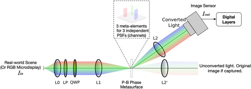
Research Article                                                              Vol. 60, No. 15 / 20 May 2021 / Applied Optics     4357

phase also has its handedness changed [22,24]. The power ratio
between light imbued with this geometrical phase and the total
incident light is a function of frequency, and this function is
referred to as the polarization conversion efficiency (PCE) [25].
   Given a target convolution layer to be implemented opti-
cally, we purposely design the metasurface such that each of the
meta-elements in a given unit cell has a unique PCE spectrum
that responds to only one specific, very narrow frequency band       Fig. 1. Comparing our proposed system with conventional systems,
corresponding to a particular input channel. In this way, meta-      our system moves the first layer of a DNN into the optical domain
surfaces let us apply different phase profiles to different input    based on novel metasurface-based designs. This hybrid system allows
channels, which enables the system to have different PSFs for        us to use a simple monochromatic sensor while completely eliminating
each channel, which effectively allows processing multi-channel      the image signal processor (ISP), which is power-hungry and on the
inputs.                                                              critical path of the traditional pipeline. (a) Existing DNN-based vision
                                                                     system pipeline and (b) our proposed optical-electrical hybrid vision
   However, using metasurface optics for optical deep learning       pipeline.
is not without challenges. Determining the metasurface param-
eters to produce a given PCE specification, known as the inverse
design problem of a metasurface, is known to be extremely
time-consuming, because it involves exploring billions of design        • We are the first to address generic (multi-channel) con-
points, each of which requires simulating the time evolution         volution in free-space optics. This is achieved by a novel use of
of the system by computing solutions to Maxwell’s equations          metasurface optics to independently modulate the phase that is
[26,27]. Second, an optical layer when directly plugged into a       imparted to different frequency components of incident light.
DNN model will likely not match the exact results of the math-          • We present an end-to-end differentiable optimization
ematical convolution due to optical design imperfections and         framework, which allows us to co-train the optical parameters
sensor artifacts (e.g., noise).                                      and digital layer parameters to maximize the overall accuracy
   We propose an end-to-end optimization framework that              and efficiency.
avoids the inverse design problem altogether while minimizing           • We evaluate our system on multiple vision networks
the overall network loss. We start from existing meta-element        (AlexNet, VGG, and ResNet50). Our simulation results show
designs whose PCEs are close enough to our desired PCE speci-        that our system can reduce the overall system energy by up to an
fications. We then accurately model the metasurface behaviors
                                                                     order of magnitude while sacrificing an accuracy loss of 1.9% on
to integrate the metasurface into an end-to-end design frame-
                                                                     average (0.8% minimum).
work, which co-optimizes the metasurface design with the
rest of the network including the analog sensor and the digital
layers in a DNN model. Critically, the end-to-end pipeline is
differentiable, which allows us to generate a complete system        2. RELATED WORK
design (metasurface optical parameters and the digital layer         A. Integrated Photonics DNN
parameters) using classic gradient descent methods.
                                                                     Existing optical deep learning systems take two major
                                                                     approaches: integrated photonics [28–30] and free-space optics
C. Contributions                                                     [16–18,31]. Burgos et al. [32] propose a multi-layer perceptron
Leveraging the end-to-end design framework, we explore a             (MLP) implementation based on microring resonators (MRRs)
system where the first layer in a DNN is moved to the optical        [33]. Other implementations used different optical mechanisms
domain; the image sensor captures the convolutional layer’s out-     such as Mach–Zehnder interferometers (MZIs) [28,30], but
put feature map, which is then processed in the digital domain       the general principle holds. Integrated photonics circuits are
to finish the entire network. Figure 1 illustrates the idea of our   fundamentally designed to execute matrix multiplications.
system.                                                              Convolutions must be first converted to matrix multiplication
   Our design has three advantages. First, since the sensor cap-     and then mapped to the photonics substrate [30].
tures the feature map rather than the original RGB image, our           The advantages of integrated photonics is that it could be
system enables us to use a simple monochromatic sensor rather        directly integrated into CMOS chips, to minimize the form
than a RGB sensor used in conventional systems, eliminating          factor. Integrated photonics could potentially enable optical
engineering efforts of many components such as the color filter      training [34]. The disadvantage of integrated photonics is
array (CFA).                                                         twofold. First, they fundamentally require coherent light (gen-
   Second, since we use a monochromatic sensor that captures         erated from a laser source) and, thus, could not directly operate
the output feature map, we can avoid the often power-hungry          on real-world scenes, where light is incoherent. Second, due to
computations in the image signal processor (ISP), which is           the quadratic propagation losses of integrated waveguides, the
required by conventional RGB sensors to correct sensor artifacts     power consumption of the integrated photonics system could
such as demosaicing and tone mapping. Avoiding ISP leads to          be extremely high when implementing realistic DNN models
significant overall energy reduction.                                [32]. The power goes up to 500 W to execute an MLP layer with
   Finally, by moving the first layer into optics, we reduce the     105 neurons, which in turn limits the scale of the DNN to be
amount of computation left in the digital domain.                    implemented.
   In summary, this paper makes the following contributions: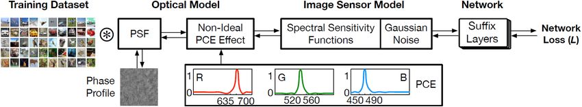
4358     Vol. 60, No. 15 / 20 May 2021 / Applied Optics                                                    Research Article

B. Free-Space Optical DNNs
Motivated by the limitations of integrated photonics, recent
research has started exploring free-space optics, which exploits
the physical propagation of light in free space through a custom
lens to perform convolution. Chang et al. [16] demonstrate
a 4- f system using DOEs to implement convolution layers,
which supports multiple output channels but does not support         Fig. 2.   Typical “4- f ” system.
multiple input channels. Lin et al. [17] proposes a DOE-based
free-space design, which supports a unique network architecture         Free-space imaging scenarios can be modeled by assuming
that is neither an MLP nor a convolutional neural network            spatially incoherent light and a linear, shift-invariant optical
(CNN): it consists of the basic structures of an MLP but has a       system. Under these assumptions, the image formed by an opti-
limited receptive field typically found in CNNs. Miscuglio et al.    cal system (Iout ) can be modeled as a convolution of the scene,
[19] demonstrate a 4- f system where a DMD is placed in the          i.e., input signal (Iin ), with the PSF of the optical system [11]:
Fourier plane to implement the convolutional kernels of a CNN
layer by modulating only the amplitude of the incident light.                   Iout (x , y , ω) = Iin (η, ξ, ω) ? PSF(η, ξ ),       (1)
However, this system is also limited to only being able to process
single-channel inputs.                                               where ? denotes convolution, Iin (η, ξ, ω) denotes the intensity
                                                                     of input pixel (η, ξ ) at frequency ω, and Iout (x , y , ω) denotes
                                                                     the intensity at output pixel (x , y ) at frequency ω.
C. Deep (Computational) Optics                                          An optical convolution system is typically implemented
Implementing deep learning (convolution) in free-space optics        using a so-called “4- f ” system [11] as illustrated in Fig. 2,
is reminiscent of classic computational optics and compu-            which consists of two lenses, each with focal length f . The first
tational photography, which co-designs optics with image             lens is placed one f away from the object plane, producing a
processing and vision algorithms [35]. Recent progresses in deep     Fourier plane another f after the first lens. The second lens is
learning has pushed this trend even further to co-train optical      placed another f from the Fourier plane, producing an inverted
parameters and DNN-based vision algorithms in an end-to-             conjugate image plane, which is in total 4- f from the original
end fashion. Examples include monocular depth estimation             object plane. An image sensor is placed at the image plane to
[36–39], single-short high dynamic range imaging [40,41],            capture the output for future processing (e.g., activation and
object detection [36], super-resolution, and extended depth of       subsequent layers) in the electronic domain. The reason why
field [42].                                                          the back focal plane of the first lens is referred to as the Fourier
                                                                     plane is because the electric field on that plane can be expressed
D. Computing in Metasurface Optics                                   in terms of the Fourier transform of the electric field on the
                                                                     front focal plane. Mathematically speaking, let Ui (η, ξ ) be
Lately, metasurface optics have been used for various computa-       the field in the input plane of the 4- f system, where (η, ξ )
tion tasks through co-optimizing optics hardware with backend        denote the spatial coordinates in that plane. Also, let U F (u, v)
algorithms. Lin et al. [43] uses a simple ridge regression as an     be the field in the Fourier plane of the 4- f system, where (u, v)
example backend while our work employs a neural network. Lin         denote the spatial coordinates in that plane. Then, the field in
et al. focuses on exploiting full-wave Maxwell physics in small      the Fourier plane is expressed in terms of the field in the input
multi-layer 3D devices for non-paraxial regime and enhanced          plane as
spatial dispersion, spectral dispersion, and polarization coher-
                                                                                                                   v

ence extraction. In contrast, our work focuses on exploiting                                                 u
                                                                                       U F (u, v) = Fi           ,      ,             (2)
large-area single-layer metasurfaces for computer vision tasks.                                             λf λf
   Colburn et al. [44] used metasurfaces for convolution, too.
To support multiple input channels, however, they use three          where λ is the wavelength of the incident light, f is the focal
separate laser sources, each going through a separate 4- f system,   length of the lenses in the 4- f system, and Fi ( f η , f ξ ) is the
whereas we leverage polarization to support multiple input           Fourier transform of Ui (η, ξ ), with ( f η , f ξ ) denoting spatial
channels with one 4- f system, potentially simplifying the           frequency components.
design and the overall form factor of the system.                       The PSF of the optical system is dictated by the phase mask
                                                                     placed at the Fourier plane. The phase mask alters the PSF
                                                                     by imparting a certain phase change to the incident light.
3. FUNDAMENTALS OF FREE-SPACE OPTICS                                 It achieves this by introducing a phase term to the field
A typical setup for a free-space optical DNN is similar to com-      on the Fourier plane, meaning it multiplies U F (u, v) by
putational cameras [35,45], where a custom-designed lens             exp(i8(u, v)) (here the imaginary unit is denoted as i). The
directly interrogates the real-world scene as an optical input       phase change induced by a phase mask is called the phase mask’s
signal. The lens executes the first convolution or fully connected   phase profile, which is often determined by the geometric prop-
layer of a DNN; the layer output is captured by an image sensor      erties of the meta-elements on the phase mask (e.g., dimension,
and sent to the digital system to execute the rest of the DNN        orientation, thickness). Our goal is to find the phase profile 8
model. This setup is a natural fit for machine vision applications   to generate a PSF that matches a target image that contains the
where the inputs are already in the optical domain and have to be    intended convolution kernel W. This can be formulated as an
captured by a camera sensor anyways.                                 optimization problem: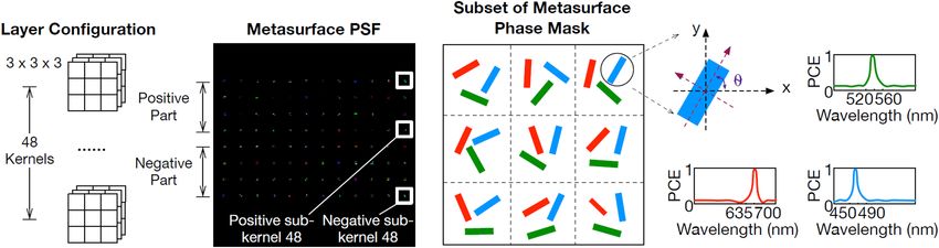
Research Article                                                                              Vol. 60, No. 15 / 20 May 2021 / Applied Optics    4359

                             min kW − PSF(8)k.                                 (3)    an anisotropic meta-element [46]. Specifically, a meta-element
                               8
                                                                                      that is geometrically symmetric with respect to its main axes
   Without the phase mask, the image captured by the image                            and that has an in-plane orientation angle θ induces a geometric
sensor simply reproduces the input Iin . With the optimized                           phase 2θ on the incident light [46,47]. Therefore, for a phase
phase mask, the output image is naturally the result of the                           mask that consists of M × N meta-elements, each having an
convolution in Eq. (1).                                                               in-plane rotation of θm,n , the phase profile 8 of the phase mask
   The output of a generic convolutional layer is given by                            is also an M × N matrix, where each element is 2 × θm,n .
                                                                                          In a 4- f system (with a DOE or a metasurface), the PSF
                   C in
                   X                                                                  relates to the phase profile (8) of the phase mask according to
  j
Iout (x ,   y) =          Iini (x , y ) ? W j ,i (x , y ),   ∀ j ∈ [1, C out ]. (4)   the following equation:
                   i=1
                                                                                                          PSF(8) = |F −1 {e i8 }|2 ,                   (5)
   The optical convolution in Eq. (1) can be seen as a simplifi-
cation of Eq. (4) whenever the number of input channels (C in )                       where F −1 denotes the inverse 2D Fourier transform and
and the number of output channels (C out ) of the convolutional                       e i8 acts as the system’s transfer function [11]. Thus, find-
layer are both equal to 1. Supporting multiple output channels                        ing the optimal phase profile is formulated as the following
(i.e., multiple convolution kernels) is achieved by designing                         optimization problem:
a PSF that spatially tiles the C out convolution kernels on the
same plane; each tile corresponds to a convolution kernel W j ,·                                       min kWk − |F −1 {e i8k }|2 k2F ,                (6)
                                                                                                        8k
[16]. As the input image is convolved with the system’s PSF, it
is naturally convolved with the different convolution kernels,                        where k · k F denotes the Frobenius norm, Wk denotes the k th
effectively generating multiple output channels.                                      channel of the target PSF that encodes the convolution kernels,
   However, supporting multiple input channels is a fundamen-                         and 8k denotes the discretized 2D phase profile of channel k.
tal challenge unaddressed in prior work. Essentially, the optical                        When performing the phase optimization process, we use a
system must have multiple PSFs, each of which must apply to                           discretized version of the target PSF, encoding it in a numerical
only a particular frequency (i.e., channel) of the incident light.                    array of N × N pixels. During this phase optimization process,
This is inherently unattainable in prior works that use DOEs
                                                                                      we iteratively update the numerical array 8k of N × N pixels
[21] to implement the phase mask. This is because the phase
                                                                                      that contains the phase profile. The optimization process has
profile that is implemented for one frequency is a scalar multiple
                                                                                      the objective of making the PSF yielded by 8k to be as close as
of the one that is implemented for other frequencies. As such,
                                                                                      possible to the target PSF that encodes Wk . Once we obtain the
it is not possible to create independent phase profiles for the
                                                                                      optimized numerical array 8k , we can do the mapping between
different frequency components of incident light. To overcome
                                                                                      the (row, column) positions in the numerical phase array and
this limitation, we instead propose to implement the phase mask
                                                                                      (u, v) positions in the plane of the phase mask. For this, we
using geometrical phase metasurfaces, which we describe in
                                                                                      remember that each point (u, v) in the Fourier’s plane (where
detail next.
                                                                                      the phase mask lies) is associated with a point ( f η , f ξ ) in
                                                                                                                                                       the
                                                                                      frequency space domain given by ( f η , f ξ ) = λuf , λvf , as
4. METASURFACE-BASED OPTICAL
                                                                                      can be seen in Eq. (2). Additionally, we know that the largest
CONVOLUTION
                                                                                      (absolute value of ) spatial frequency component of the input
The goal is to design the phase mask in a way that different                          image that makes it into the Fourier plane is given by one half of
PSFs are applied to different input channels. Unlike DOEs                             the sampling rate of the display in the input plane, known as the
that modulate only the phase of the incident light by applying                        Nyquist rate [11]. That is,
a propagation phase, metasurfaces are able to also introduce
a geometrical phase. Our key idea is to use different kinds of                                                                         1
                                                                                                          | f η |max = | f ξ |max =      ,             (7)
meta-elements that imbue a geometrical phase to incident light                                                                        2d
of different frequency components. That way, the metasurface                          where d is the pixel pitch of the display in the input plane that
introduces different phase profiles to each of the frequency com-                     projects the input image into the optical system. Given this,
ponents (channels) of incident light. In the following, we first                      the size of the spatial frequency domain is 1/d , and, since the
describe the phase modulation assuming only one input channel                         phase mask needs to cover it all, the size of the phase mask needs
and then discuss the case with multiple input channels, which
                                                                                      to be λdf . We then divide the region of λdf × λdf into N × N
allows us to attain generalized free-space optical convolution
                                                                                      subregions (or “pixels”). Thus, the size of these “phase pixels” is
with multiple input and output channels.
                                                                                      given by

A. Single-Channel Case                                                                                                     λf
                                                                                                                  1u =        .                        (8)
                                                                                                                           Nd
Our metasurface phase mask consists of a set of meta-elements,
each of which induces a particular phase change to the incident                          After we have obtained the numerical values of the elements
light. Physically, we use the Pancharatnam–Berry (P–B) phase                          in the optimized 8k array, we simply divide them by 2 to obtain
[22,24]. P–B phase comes from the spin rotation effect that                           the value of the in-plane orientation of each meta-element
arises from the interaction between circularly polarized light and                    on the metasurface. We would like to note that the objective
4360      Vol. 60, No. 15 / 20 May 2021 / Applied Optics                                                                       Research Article

Fig. 3. Target PSF for a convolutional layer that has 48 kernels, where each kernel has three channels and each channel has 3 × 3 elements. The
PSF is arranged as 12 × 8 tiles, with one positive and one negative tile for each kernel. Each tile is 3 × 3. Each tile has three channels, corresponding
to different frequencies of incident light. On the metasurface, each meta-element has a unique in-plane rotation θ. Each unit cell in the metasurface
contains three kinds of meta-elements with distinct geometric parameters, and each kind is associated to a different channel. Following Eq. (5), all the
meta-elements associated to the same channel collectively form a phase mask that shapes the PSF for that channel, which matches the correspond-
ing channel of the convolution kernels. Meta-elements associated to the same channel have the same PCE spectrum, and, in the ideal case, the corre-
sponding PSF is applied to the associated input channel only, without cross talk.

function in Eq. (6) is differentiable. Thus, phases (and, there-                pixels for all channels will be larger than the size of the metasur-
fore, the values of the meta-elements’ orientations) could be                   face’s unit cells (the former being in the order of microns, and
co-optimized with the rest of DNN in an end-to-end fashion, as                  the latter being in the order of hundreds of nanometers). This
we will show in Section 5.                                                      means that the phase pixels of any given channel are filled with
   Now, we will discuss how we design the target PSF that                       multiple unit cells (each of which contains one of each kind of
encodes the network’s convolution kernels. Since PSF physically                 meta-element associated to the different channels). Since the
corresponds to light intensity [11] and there is no negative light              orientation of each meta-element in the unit cell is independent
intensity, the negative values in a kernel cannot be physically                 to that of the others, we can essentially multiplex the phase pro-
implemented. A mathematical explanation is that the PSF is                      files associated to the different channels on the same metasurface
the square form of an expression, as shown in Eq. (5), and, thus,               without issues.
must be nonnegative. To address this limitation, we use the idea                    The remaining challenge is making sure that the PSF that
of Chang et al. [16] by splitting a kernel into two sub-kernels: one            is yielded by the set of meta-elements of one kind should only
contains only the positive portion, and the other contains only                 be applied to light of the corresponding channel (frequency
the (absolute value of the) negative portion of the kernel. The                 component) in order to correctly implement the convolution
final kernel is calculated by subtracting the negative sub-kernel               layer. That is, we must minimize cross talk effects that make
from the positive sub-kernel.                                                   meta-elements apply the geometrical phase to a portion of the
   As a result, for a layer that has K kernels, the target PSF con-             light of the other channels. We make use of the fact that each
tains 2K tiles that are used to represent these kernels. Figure 3               meta-element acts as a phase retarder, which makes a portion
shows the target three-channel PSF for a layer that has 48 ker-                 of incident circularly polarized light change its handedness and
nels, each of dimension 3 × 3 × 3. The PSF has 96 tiles, where                  get imbued with a geometrical phase. This portion is dependent
the ones in the top half are the positive sub-kernels, and the ones             on the wavelength of incident light and is the PCE. Effectively,
in the bottom half contain the sub-kernels. Each tile is 3 × 3,                 when incident light from the input image interacts with the
which corresponds to the 3 × 3 elements in one channel of a                     set of meta-elements that has a given PCE spectrum, the cor-
three-channel sub-kernel. In order to yield this target PSF, the                responding intensity profile in the output plane (given by the
in-plane rotation of every meta-element on the metasurface is                   convolution between the input intensity profile and the PSF
optimized from Eq. (6). The three meta-elements in a unit cell                  yielded by this set of meta-elements) is weighted by PCE(ω) at
of the metasurface are used to yield the three channels of the                  frequency ω. With the PCE taken into account, the contribu-
target multi-channel PSF, which we discuss next.                                tion of intensity in the output (capture) plane that is attributed
                                                                                to an input channel c can be expressed as
B. Multi-Channel Case                                                                                 C in
                                                                                                      X             0          0
With what was discussed above, we are able to use the in-plane                    c
                                                                                 Icon (x , y , ω) =            PCEc (ω)(PSFc (η, ξ ) ? Iinc (η, ξ, ω)),
rotations of the meta-elements to engineer the PSF to match                                           c 0 =1
any given 2D matrix (i.e., a channel in the target kernel). When                                                                              (9)
going from the single-channel case to the multi-channel case,                   where channel c of the input image is affected by the PSF c 0
we first note that the size of the “phase pixels” will depend on                yielded by the different meta-element sets in the metasurface,
the wavelength λ according to Eq. (8). This means that the                      which is where the sum over PSF channels c 0 comes from.
pixels (regions in the metasurface that impart a given phase value                 In the ideal case, the PCE is a delta function that is 1 for
to incident light) associated with different channels will have                 a very narrow band, e.g., red wavelength, and 0 for all other
different sizes. We address this by noting that for our choice for              wavelengths. That way, the PSF carried by the meta-elements
the values of f , d , and λ range, the size of the metasurface phase            will effectively convolve only with one particular input channel.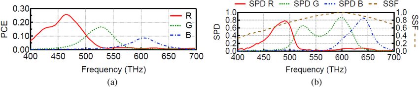
Research Article                                                                            Vol. 60, No. 15 / 20 May 2021 / Applied Optics         4361

Figure 3 shows an example that supports three input channels                                        Iinc (x , y , ω) = SPDc (ω)Iinc (x , y ),           (10)
(e.g., natural light from the real-world). The key is that each
unit cell consists of three meta-elements, each carrying a unique                 where SPD (ω) is the spectral power distribution (SPD) of
                                                                                                c

                                                                                  color channel c in the input light at frequency ω, and Iinc (x , y ) is
PCE. When white light containing the RGB wavelengths
                                                                                  the light intensity of pixel (x , y ) in channel c and is directly read
(channels) is incident on the phase mask, the red channel will
                                                                                  from the RGB image in the training data.
acquire the phase imparted by the meta-element associated to
                                                                                     In the forward pass during training (and also inference), the
the red channel only, mimicking the convolution between the
                                                                                  PSF generated from the phase profile (8) is first convolved
red channel of the input and the corresponding PSF; the same
                                                                                  with the input image from a training dataset under the impact
process applies to green and blue wavelengths as well. The out-
                                                                                  of the PCE as described by Eq. (9). The convolution output is
put is naturally the superposition (sum of intensity) of the three                captured by the image sensor, which we model by its spectral
convolution outputs.                                                              sensitivity function (SSF). In addition, image sensors intro-
   In reality, the metasurface design is regulated by fabrication                 duce different forms of noise, which we collectively model as a
constraints and, thus, the actual PCE will never be an ideal delta                Gaussian noise function N(µ, σ 2 ), based on the central limit
function, which leads to cross talk, i.e., the PSF of a channel i                 theorem. In order to retain the behavior of optical shot noise,
will be convolved with input channel j . Therefore, it is critical                which is proportional to the number of incident photons, we
to optimize the end-to-end system to minimize the impact of                       programmed the noise layers on our DNN to have a standard
cross talk, which we discuss next.                                                deviation σ that is proportional to the magnitude of those layers’
                                                                                  inputs.
                                                                                     As a result, the output signal yielded by the sensor is given by
5. END-TO-END TRAINING FRAMEWORK
                                                                                                       C in Z
Figure 4 shows the end-to-end system setup, from light in the                                          X
real-world scene (or equivalently a RGB microdisplay) to the                         Iout (x , y ) =                        c
                                                                                                                     SSF(ω)Icon (x , y , ω)dω + N(µ, σ 2 ).
                                                                                                       c =1
network output. It consists primarily of three components:
                                                                                                                                                 (11)
a metasurface-based optical system that implements the first
                                                                                     Note that the sum across different input channels, required
convolution layer of a DNN, an image sensor that captures the
                                                                                  by correctly implementing a convolution layer, is realized in
output of the optical convolution, and a digital processor that                   our design “for free” by superimposing the intensity profile of
finishes the rest of the network, which we call the “suffix layers.”              the different frequency components that are incident on the
   In order to maximize the overall network accuracy, we co-                      detector. The total light intensity at the output plane is naturally
optimize the optical convolution layer with digital layers in                     the (weighted) sum of the intensities of individual channel
an end-to-end fashion. Figure 5 shows the end-to-end dif-                         components.
ferentiable pipeline, which incorporates three components:                           Plugging Eq. (10) into Eq. (9) and plugging Eq. (9) into
an optical model, a sensor model, and the digital network.                        Eq. (11) yields the sensor output, which becomes the input to
The phase profile (8) in the optical model and the suffix layer                   the digital suffix layers to then produce the network’s output and
weights (W) are optimization variables. The loss function L that                  loss. The sensor output can then be expressed as
is used to measure this system’s performance is the same as what
                                                                                                   C in
                                                                                                        " C Z
can be used with a conventional all-digital neural network, like                                           in
                                                                                                   X     X                       0
the log loss function.                                                             Iout (x , y ) =                 SSF(ω)PCEc (ω)SPDc (ω)dω
   The input to the system is light, which in practical applica-                                       c        c0

tions are from the real-world scene. In our work, we envision a                                                            #
RGB microdisplay displaying images from datasets to emulate                                                     c0
                                                                                                    × PSF (η, ξ ) ? Iinc (η, ξ ) + N(µ, σ 2 ).
the real-world scene as is done in prior work [16]. Thus, channel
c in the input is expressed as                                                                                                                          (12)

Fig. 4. Hardware system. Light from the real-world (or a microdisplay) is collimated by lens L0, and then goes through a linear polarizer (LP) and a
broadband quarter-wave plate (QWP) so that light becomes circularly polarized. The plane of the LP is the input plane of the 4- f system. A metasur-
face phase mask is placed at the Fourier plane. A portion of the light gets the engineered phase shift and has its polarization handedness switched. This
“converted” portion of the light gets sent to lens L2, via a phase “grating” [48] added to the phase profile, while the unconverted light is sent to lens L2’
on the optical axis. L2 is at a distance f from the metasurface. Finally, light is detected by the image sensor placed at a distance f after L2.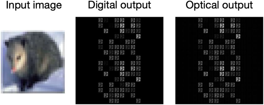
4362      Vol. 60, No. 15 / 20 May 2021 / Applied Optics                                                             Research Article

Fig. 5. End-to-end training framework. The polarization conversion efficiency profile is network-independent and is obtained from real meta-
surface optics fabrications. The phase profile can be optimized using the training data and fine-tuned with the DNN model suffix layers (i.e., layers
implemented in the digital domain) together in an end-to-end fashion.

   The above expression can be simplified into the following                  tiles of different convolution kernels and of different channels
form:                                                                         within a kernel are tiled in a 2D plane (Fig. 3). Second, since
                C in
                     "C
                        in
                                              #                               the monochromatic sensor integrates the intensity of all inci-
                X     X
Iout (x , y ) =                       c0
                           A c 0 c PSF (η, ξ ) ? Iinc (η, ξ ) + N(µ, σ 2 ),   dent frequency components, this naturally emulates the sum
                c     c0                                                      over channels that needs to be performed when calculating the
                                                                (13)          output of a digital convolutional layer, as described by Eq. (4).
                                 0
where A c 0 c = SSF(ω)PCEc (ω)SPDc (ω)dω, and we can
                 R
define a cross talk matrix whose elements are A c 0 c for the differ-
ent values of c 0 and c . Note that the convolution layer mapped              6. EVALUATION
to metasurface, as described by Eq. (11), is differentiable, and,             A. Methodology
thus, enables end-to-end training using classic gradient descent-             1. Networks and Datasets
based optimization methods. In doing so, the suffix layers can
be optimized to compensate for the effects introduced by cross                We implement the end-to-end training framework in
talk. During backpropagation, the phase profile (8) and the                   TensorFlow. We differentiate the metasurface optics layer
digital layer weights (W) are optimized. Note that the PCEs of                (from phase profile to the target kernel) and integrate the dif-
the meta-elements are network-independent and are directly                    ferentiation into the backpropagation process. We evaluate on
obtained from fabrication. They are kept fixed throughout                     three networks: AlexNet [49], VGG-16 [50], and ResNet50
training.                                                                     [51], all on the CIFAR-100 dataset [52].

A. Practical Considerations                                                   2. Training Details

Since different sub-kernels are tiled together for the ease of train-         To accelerate convergence, we first train the entire network
ing, the outputs of different sub-convolutions (i.e., convolution             in three separate steps: (1) train the entire network digitally,
between a sub-kernel and the corresponding channel in the                     (2) use the first layer’s weights to optimize the phase mask,
input) will be tiled too. We must make sure that the different                and (3) finally the optimized phase mask and the pre-trained
sub-convolution outputs do not overlap so that we can assemble                suffix layers are then fine-tuned end-to-end until convergence.
them (digitally) to form the actual convolution output. To that               The phase optimization process consists of running a gradi-
end, we pad each sub-kernel with space between cells in the                   ent descent algorithm to minimize the loss function shown in
phase mask. For instance, in the illustrative example shown                   Eq. (6). In Supplement 1, we provide further details about the
in Fig. 3, we pad each 3 × 3 sub-kernel by 8 pixels each side                 derivation of the expression of the gradient of this function, as
to form a 19 × 19 matrix, effectively separating neighboring                  well as a way for it to be computed efficiently. In all networks,
sub-kernels in the phase mask by 16 pixels. In our work, we                   the results converge after 2000 iterations of the gradient descent
pad the sub-kernels by 20 pixels each side to form a 43 × 43                  cycle. The phase masks and suffix layers’ parameters are then
matrix, effectively neighboring sub-kernels by 40 pixels. In                  end-to-end fine-tuned with the suffix layers for 50, 150, and 50
summary, given the kernels in a target convolution layer, we first            epochs for AlexNet, VGG, and ResNet, respectively.
separate each kernel into two sub-kernels, tile all the sub-kernels
on the same plane, and then add padding to form the actual                    3. Hardware Modeling Details
target PSF matrix, for which we then apply the phase optimiza-
tion described in Eq. (6) to derive the required phase profile                The metasurface designs we use are from Wang et al. [25], who
and, thus, the in-plane rotation of each meta-element on the                  provide the detailed design specifications of three kinds of
metasurface.                                                                  meta-elements, each of which is designed to have its highest
                                                                              response at red, green, and blue bands of the visible spectrum.
                                                                              The meta-elements are pillars made out of Si, with a height
B. Monochromatic Sensor                                                       of 320 nm, sitting on a SiO2 substrate. These meta-elements
It is important to note that our system design lets us use a sim-             have a rectangular cross section whose dimensions depend
ple monochromatic sensor rather than a conventional RGB                       on the channel each meta-element is associated with. Meta-
sensor. This is because of two reasons. First, the results of all             elements associated with the red channel have a cross section
output channels lie completely within a 2D plane because the                  of 145 nm × 105 nm, those associated with the green channel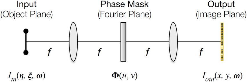
Research Article Vol. 60, No. 15 / 20 May 2021 / Applied Optics 4363
Fig. 6. Parameters of hardware components. We use these to compute the cross talk matrix, which is necessary to account for the effects of the cross
talk between channels. (a) PCEs of the three meta-elements designs and (b) the spectral power distributions of the microdisplay and the spectral sensi-
tivity function of the image sensor modeled in our computational experiments.
have a cross section of 110 nm × 80 nm, and those associated
with the blue channel have a cross section of 90 nm × 45 nm. A
unit cell of the metasurface is 420 nm × 420 nm and contains
the three kinds of meta-elements on it. Based on these design
specifications, we run the well-known MEEP package [53,54]
for electromagnetics simulations to generate the corresponding
PCEs of the three kinds of meta-elements, which we use in our
design and simulation. Figure 6(a) shows the PCE of the three
kinds of meta-elements. While the PCEs are not ideal delta Fig. 7. Comparison between the output of a convolution layer
functions, they do provide the highest responses in distinct when implemented digitally, and when implemented optically. The
bands. optical output is simulated, taking the effects of cross talk between
We use the Sony ICX274AL image sensor, whose SSF we channels into account.
adapt from the design specification [55]. We use the eMagin
OLED-XL RGB microdisplay from eMagin, whose SPDs we
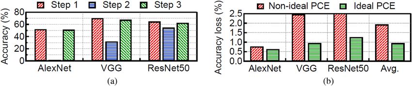
obtained by contacting the display manufacturer. Figure 6(b) accuracy loss. Overall across the three networks, our optical-
shows the normalized SPDs of the microdisplay pixels (left y electrical DNN system leads to on average only an 1.9% (0.8%
axis) and the SSF of the sensor (right y axis). Comparing the minimum) accuracy loss compared to fully digital networks.
SPDs and the PCEs in Fig. 6, the PCE and SPD peaks are close The accuracy loss could be further improved if we could improve
to each other (e.g., both the red PCE and the red light from the the PCE of the metasurface designs. Figure 8(b) compares the
microdisplay peak at around 450 THz to 500 THz). We use accuracy loss on the three networks between using ideal PCEs
these PCE and SPD functions to calculate the cross talk matrix, (i.e., delta functions) and non-ideal PCEs (from actual designs,
which is a necessary part in the system’s optimization process so used in Fig. 8(a). Using an ideal PCE leads to an average accu-
that it can account for cross talk effects. racy loss of only 0.9%. This suggests that our system design can
readily benefit from better metasurface designs in the future.
B. Network Accuracy and Efficiency
3. Efficiency
1. Phase Optimization
We find that our phase optimization allows us to generate a PSF Our system reduces the overall computational cost in two ways.
that resembles the target kernel. The loss decreases by 2 to 3 First, we completely avoid the need to process raw sensor data
orders of magnitude from its initial value after 2000 iterations, using the power-hungry ISP. Traditional vision systems use ISPs
reaching convergence. Figure 7 compares the output feature to process raw sensor data (e.g., demosaic, tone mapping) to
map of the first layer between the digital implementation and generate RGB images for the DNN to process, but, since in our
the optical implementation, which match well, indicating that system the image sensor captures the output feature map rather
the optical output provides a desirable input to the suffix digital than the RGB image, the ISP processing could be avoided.
layers. Note that the different output channels are tiled in one We measure the power of the Nvidia’s Jetson TX2 board,
2D plane. which is representative of today’s high-end systems for mobile
vision [56]. The ISP consumes about 0.5 mJ of energy to gen-
erate one RGB frame. In contrast, the energy consumed to
2. Accuracy execute AlexNet, VGG, and ResNet50 on a Google TPU-like
We find that our end-to-end design leads to little accuracy loss. specialized DNN processor [9] is 0.31 mJ, 0.36 mJ, 0.05 mJ,
Figure 8(a) shows the network accuracies of the three training respectively, which we estimate using a recent DNN energy
steps. As we can see, step 1 is the original network executed fully modeling framework [57,58]. Avoiding the ISP yields 2.4× to 1
in the digital domain and generally has the highest accuracy. order of magnitude energy saving.
Step 2 optimizes the PSF from the target convolution kernel Secondarily, by pushing the first CNN layer into the opti-
and directly integrates the optimized PSF into the network; this cal domain, we also reduce the total amount of computations
leads to significantly lower accuracy. However, after end-to-end (measured in the number of multiply accumulate, or MAC,
fine-tuning with the suffix layers, we could largely gain the operations) to compute the DNN. In AlexNet, the MAC saving4364 Vol. 60, No. 15 / 20 May 2021 / Applied Optics Research Article
Fig. 8. Accuracy results obtained after running the pipeline on different datasets. (a) Accuracy comparison using metasurface designs and (b) accu-
racy loss of step 3 (our design) from step 1 (fully digital) when using ideal and non-ideal PCEs.
is 4.4%, and the MAC saving is 0.8% and 0.5% for ResNet50 5. L. Bertinetto, J. Valmadre, J. F. Henriques, A. Vedaldi, and P. H.
and VGG, respectively. Torr, “Fully-convolutional Siamese networks for object tracking,”
in European Conference on Computer Vision (Springer, 2016),
pp. 850–865.
7. DISCUSSION AND CONCLUSION 6. H. Chen, O. Engkvist, Y. Wang, M. Olivecrona, and T. Blaschke, “The
rise of deep learning in drug discovery,” Drug Discov. Today 23(6),
This paper demonstrates the first free-space optics approach that 1241–1250 (2018).
enables general convolutional layers. The significance of our 7. Y. LeCun, J. S. Denker, and S. A. Solla, “Optimal brain damage,” in
system is threefold. First, it eliminates the need for the power- Advances in Neural Information Processing Systems (1990), pp. 598–
605.
hungry ISP. Second, it simplifies the sensor design and enables
8. S. Han, H. Mao, and W. J. Dally, “Deep compression: compressing
the use of a simple monochromatic sensor rather than a RGB deep neural networks with pruning, trained quantization and Huffman
sensor. Finally, it reduces the computation to execute a DNN. coding,” International Conference on Learning Representations
Overall, we show an order of magnitude of energy saving with (ICLR), San Juan, Puerto Rico, 2–4 May 2016.
1.9% on average (0.8% minimum) accuracy. 9. N. P. Jouppi, C. Young, and N. Patil, et al., “In-datacenter perform-
We are in the process of fabricating an optical prototype. ance analysis of a tensor processing unit,” in ACM/IEEE 44th Annual
International Symposium on Computer Architecture (ISCA) (IEEE,
While our current design pushes only the first DNN layer
2017), pp. 1–12.
into optics, pushing more layers into optics is possible but 10. Y.-H. Chen, J. Emer, and V. Sze, “Eyeriss: a spatial architecture
not without challenges. The key challenge is that it is difficult for energy-efficient dataflow for convolutional neural networks,”
to optically implement non-linear functions, which usually SIGARCH Comput. Archit. News 44, 367–379 (2016).
have to be implemented in the electrical domain, introducing 11. J. W. Goodman, Introduction to Fourier Optics (Roberts and
Company, 2005).
optical-electrical interface transduction overhead. Therefore,
12. N. H. Farhat, D. Psaltis, A. Prata, and E. Paek, “Optical implementa-
a future direction is to comprehensively explore the hybrid tion of the Hopfield model,” Appl. Opt. 24, 1469–1475 (1985).
optical-electrical design space to evaluate the optimal partition 13. D. Psaltis, D. Brady, and K. Wagner, “Adaptive optical networks using
between optics and electronics. photorefractive crystals,” Appl. Opt. 27, 1752–1759 (1988).
14. T. Lu, S. Wu, X. Xu, and T. Francis, “Two-dimensional programmable
Funding. University of Rochester (University Research Award).
optical neural network,” Appl. Opt. 28, 4908–4913 (1989).
Acknowledgment. C. Villegas Burgos would like to thank the 15. I. Saxena and E. Fiesler, “Adaptive multilayer optical neural network
Science and Technology Council of Mexico (Consejo Nacional de Ciencia y with optical thresholding,” Opt. Eng. 34, 2435–2440 (1995).
Tecnología, CONACYT) for the financial support provided by the fellowship 16. J. Chang, V. Sitzmann, X. Dun, W. Heidrich, and G. Wetzstein, “Hybrid
they granted him. optical-electronic convolutional neural networks with optimized
diffractive optics for image classification,” Sci. Rep. 8, 12324 (2018).
Disclosures. The authors declare no conflict of interest. 17. X. Lin, Y. Rivenson, N. T. Yardimci, M. Veli, Y. Luo, M. Jarrahi, and A.
Data Availability. Data underlying the results presented in this paper are Ozcan, “All-optical machine learning using diffractive deep neural
not publicly available at this time but may be obtained from the authors upon networks,” Science 361, 1004–1008 (2018).
reasonable request. 18. J. Bueno, S. Maktoobi, L. Froehly, I. Fischer, M. Jacquot, L. Larger,
and D. Brunner, “Reinforcement learning in a large-scale photonic
Supplemental document. See Supplement 1 for supporting content. recurrent neural network,” Optica 5, 756–760 (2018).
19. M. Miscuglio, Z. Hu, S. Li, J. K. George, R. Capanna, H. Dalir, P. M.
Bardet, P. Gupta, and V. J. Sorger, “Massively parallel amplitude-only
REFERENCES Fourier neural network,” Optica 7, 1812–1819 (2020).
20. J. B. Sampsell, “Digital micromirror device and its application to pro-
1. T. Mikolov, M. Karafiát, L. Burget, J. Černocký, and S. Khudanpur,
“Recurrent neural network based language model,” in 11th Annual jection displays,” J. Vac. Sci. Technol. B 12, 3242–3246 (1994).
Conference of the International Speech Communication Association 21. D. C. O’Shea, T. J. Suleski, A. D. Kathman, and D. W. Prather,
(2010). Diffractive Optics: Design, Fabrication, and Test (SPIE, 2004), Vol. 62.
2. T. Mikolov, I. Sutskever, K. Chen, G. S. Corrado, and J. Dean, 22. N. Yu and F. Capasso, “Flat optics with designer metasurfaces,” Nat.
“Distributed representations of words and phrases and their compo- Mater. 13, 139–150 (2014).
sitionality,” in Advances in Neural Information Processing Systems 23. C. L. Holloway, E. F. Kuester, J. A. Gordon, J. O’Hara, J. Booth, and
(2013), pp. 3111–3119. D. R. Smith, “An overview of the theory and applications of meta-
3. I. Sutskever, O. Vinyals, and Q. V. Le, “Sequence to sequence surfaces: the two-dimensional equivalents of metamaterials,” IEEE
learning with neural networks,” in Advances in Neural Information Antennas Propag. Mag. 54(2), 10–35 (2012).
Processing Systems (2014), pp. 3104–3112. 24. J. P. B. Mueller, N. A. Rubin, R. C. Devlin, B. Groever, and F. Capasso,
4. J. Redmon, S. Divvala, R. Girshick, and A. Farhadi, “You only look “Metasurface polarization optics: independent phase control of arbi-
once: unified, real-time object detection,” in IEEE Conference on trary orthogonal states of polarization,” Phys. Rev. Lett. 118, 113901
Computer Vision and Pattern Recognition (2016), pp. 779–788. (2017).Research Article Vol. 60, No. 15 / 20 May 2021 / Applied Optics 4365
25. B. Wang, F. Dong, Q.-T. Li, D. Yang, C. Sun, J. Chen, Z. Song, L. Xu, in IEEE Conference on Computer Vision and Pattern Recognition
W. Chu, Y.-F. Xiao, Q. Gong, and Y. Li, “Visible-frequency dielectric (2020).
metasurfaces for multiwavelength achromatic and highly dispersive 41. C. A. Metzler, H. Ikoma, Y. Peng, and G. Wetzstein, “Deep optics for
holograms,” Nano Lett. 16, 5235–5240 (2016). single-shot high-dynamic-range imaging,” arXiv:1908.00620 (2019).
26. R. Pestourie, C. Pérez-Arancibia, Z. Lin, W. Shin, F. Capasso, and 42. V. Sitzmann, S. Diamond, Y. Peng, X. Dun, S. Boyd, W. Heidrich,
S. G. Johnson, “Inverse design of large-area metasurfaces,” Opt. F. Heide, and G. Wetzstein, “End-to-end optimization of optics
Express 26, 33732–33747 (2018). and image processing for achromatic extended depth of field and
27. S. Molesky, Z. Lin, A. Y. Piggott, W. Jin, J. Vucković, and A. W. super-resolution imaging,” ACM Trans. Graph. 37, 1–13 (2018).
Rodriguez, “Inverse design in nanophotonics,” Nat. Photonics 12, 43. Z. Lin, C. Roques-Carmes, R. Pestourie, M. Soljačić, A. Majumdar,
659–670 (2018). and S. G. Johnson, “End-to-end nanophotonic inverse design for
28. Y. Shen, N. C. Harris, S. Skirlo, M. Prabhu, T. Baehr-Jones, M. imaging and polarimetry,” Nanophotonics 10, 1177–1187 (2020).
Hochberg, X. Sun, S. Zhao, H. Larochelle, D. Englund, and M. 44. S. Colburn, Y. Chu, E. Shilzerman, and A. Majumdar, “Optical fron-
Soljačić, “Deep learning with coherent nanophotonic circuits,” tend for a convolutional neural network,” Appl. Opt. 58, 3179–3186
Nat. Photonics 11, 441–446 (2017). (2019).
29. F. Xia, M. Rooks, L. Sekaric, and Y. Vlasov, “Ultra-compact high 45. R. Ng, M. Levoy, M. Brédif, G. Duval, M. Horowitz, and P. Hanrahan,
order ring resonator filters using submicron silicon photonic wires “Light field photography with a hand-held plenoptic camera,”
for on-chip optical interconnects,” Opt. Express 15, 11934–11941 Computer Science Technical Report, CSTR 2005-02. 2, 1–11 (2005).
(2007). 46. Z. L. Deng and G. Li, “Metasurface optical holography,” Mater. Today
30. H. Bagherian, S. Skirlo, Y. Shen, H. Meng, V. Ceperic, and M. Soljacic, Phys. 3, 16–32 (2017).
“On-chip optical convolutional neural networks,” arXiv:1808.03303 47. W. T. Chen, A. Y. Zhu, V. Sanjeev, M. Khorasaninejad, Z. Shi, E. Lee,
(2018). and F. Capasso, “A broadband achromatic metalens for focusing and
31. R. Hamerly, L. Bernstein, A. Sludds, M. Soljačić, and D. Englund, imaging in the visible,” Nat. Nanotechnol. 13, 220–226 (2018).
“Large-scale optical neural networks based on photoelectric 48. C. A. Palmer and E. G. Loewen, Diffraction Grating Handbook
multiplication,” Phys. Rev. X 9, 021032 (2019). (Thermo RGL, 2002), Vol. 5.
32. C. M. V. Burgos and N. Vamivakas, “Challenges in the path toward a 49. A. Krizhevsky, I. Sutskever, and G. E. Hinton, “ImageNet classifica-
scalable silicon photonics implementation of deep neural networks,” tion with deep convolutional neural networks,” in Advances in Neural
IEEE J. Quantum Electron. 55, 1–10 (2019). Information Processing Systems (2012), pp. 1097–1105.
33. W. Bogaerts, P. De Heyn, T. Van Vaerenbergh, K. De Vos, S. K. 50. K. Simonyan and A. Zisserman, “Very deep convolutional networks
Selvaraja, T. Claes, P. Dumon, P. Bienstman, D. Van Thourhout, for large-scale image recognition,” arXiv:1409.1556 (2014).
and R. Baets, “Silicon microring resonators,” Laser Photon. Rev. 6, 51. C. Szegedy, S. Ioffe, V. Vanhoucke, and A. A. Alemi, “Inception-
47–73 (2012). v4, inception-ResNet and the impact of residual connections on
34. T. W. Hughes, M. Minkov, Y. Shi, and S. Fan, “Training of photonic learning,” in 31st AAAI Conference on Artificial Intelligence (2017).
neural networks through in situ backpropagation and gradient 52. A. Krizhevsky and G. Hinton, “Learning multiple layers of features
measurement,” Optica 5, 864–871 (2018). from tiny images,” Technical Report (Citeseer, 2009).
35. C. Zhou and S. K. Nayar, “Computational cameras: convergence of 53. A. F. Oskooi, D. Roundy, M. Ibanescu, P. Bermel, J. D. Joannopoulos,
optics and processing,” IEEE Trans. Image Process. 20, 3322–3340 and S. G. Johnson, “Meep: a flexible free-software package for
(2011). electromagnetic simulations by the FDTD method,” Comput. Phys.
36. J. Chang and G. Wetzstein, “Deep optics for monocular depth esti- Commun. 181, 687–702 (2010).
mation and 3D object detection,” in IEEE International Conference on 54. A. F. Oskooi, D. Roundy, M. Ibanescu, P. Bermel, J. D. Joannopoulos,
Computer Vision (2019), pp. 10193–10202. and S. G. Johnson, “Meep: free finite-difference time-domain (FDTD)
37. H. Haim, S. Elmalem, R. Giryes, A. M. Bronstein, and E. Marom, software for electromagnetic simulations,” 2020, https://github.com/
“Depth estimation from a single image using deep learned phase NanoComp/meep.
coded mask,” IEEE Trans. Comput. Imaging 4, 298–310 (2018). 55. Sony, “ICX274AL sensor specification,” 2020, https://www.1stvision.
38. L. He, G. Wang, and Z. Hu, “Learning depth from single images with com/cameras/sensor_specs/ICX274.pdf.
deep neural network embedding focal length,” IEEE Trans. Image 56. Nvidia, “NVIDIA Jetson TX2 Delivers Twice the Intelligence to the
Process. 27, 4676–4689 (2018). Edge,”https://developer.nvidia.com/blog/jetson-tx2-delivers-twice-
39. Y. Wu, V. Boominathan, H. Chen, A. Sankaranarayanan, and A. intelligence-edge/ (2018).
Veeraraghavan, “PhaseCam3D–learning phase masks for passive 57. Y. Feng, P. Whatmough, and Y. Zhu, “ASV: accelerated stereo vision
single view depth estimation,” in IEEE International Conference on system,” in 52nd Annual IEEE/ACM International Symposium on
Computational Photography (ICCP) (IEEE, 2019), pp. 1–12. Microarchitecture (ACM, 2019), pp. 643–656.
40. Q. Sun, E. Tseng, Q. Fu, W. Heidrich, and F. Heide, “Learning rank- 58. “Systolic-array data-flow optimizer,” https://github.com/horizon-
1 diffractive optics for single-shot high dynamic range imaging,” research/systolic-array-dataflow-optimizer.You can also read