Simulation and measurement of resonators - Uni Frankfurt

Simulation and measurement of resonators
                          Instructions for the lab course
           Supervisor: Malte Schwarz, Office: 02.410, schwarz[at]iap.uni-frankfurt.de

                                    September 2021

Information
   ˆ Unless otherwise stated by the lab course lead or supervisors, the following applies:
        – The lab course takes place on Mondays from 09:30 to 11:30 and from 12:30 to
          16:00.
        – The report must be submitted no later than two weeks after the experiment
          has been performed.
        – Please indicate all the people of your lab group in your report, as well as the
          person responsible for writing the report.
        – General information on the lab course can be found at www.linac-world.de.

Introduction
High-frequency resonators of various designs are studied at the Institute of Applied Physics
with regard to their possible applications in acceleration and focusing of charged particles.
The design process of modern particle accelerator structures is performed today to a large
extent in computer simulations, which considerably reduces the necessity to build and
measure prototypes. Both particle beam dynamics, i. e. the transformation of the ion
beam while passing through an accelerator, as well as the high-frequency properties of the
accelerating resonance structures (”cavities”) are nowadays calculated and optimized by
means of numerical methods on copmputers.
  In this experiment, resonators with simple geometry are modeled with the program CST
Microwave Studio (MWS) and the simulated results are compared with measurements.
The resonance spectrum and the Quality Factor of a cylindrical cookie box and of a bottle
are examined. The cookie box should be regarded as a model of a pillbox cavity (resp.
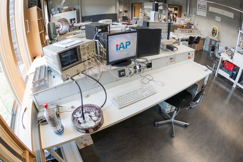
cylindrical resonator) whose modes can also be calculated analytically.

Pictures of the Experimental Setup

Figure 1: Left: Overview of the experimental setup. Right: Commercially available PET
          beverage bottle (wrapped in aluminum foil) with two coaxial connections (SMA
          connector).

Figure 2: Left: Cylindrical metal box with two coaxial ports (type-N connector). Right:
          View into the box. Capacitive (antenna on the left) and inductive (loop on the
          right) RF-coupling.

Theory
Please familiarize yourself independently with the following topics before starting the
experiment:

   ˆ Mode spectrum of cavity resonators (especially the pillbox cavity)

   ˆ How is the Quality Factor Q0 of a resonator defined (at least 2 definitions!)?

   ˆ How can Q0 be measured with the 3dB-method?

   ˆ Coupling of electromagnetic waves in resonators
         – Inductive / capacitive coupling
         – HF waves on coaxial lines and their behavior at transitions

   ˆ What are TM-/TE-modes?

   ˆ How are E- and B-fields distributed in a cylindrical cavity resonator at the lowest
     mode/resonance frequency? Where are bessel functions needed here?

   ˆ In which directions do the E- and B-field vectors point at the lowest mode/resonance
     frequency?

   ˆ What is a network analyzer (NWA)?

   ˆ What is measured with the S11- and S21-parameter?

It is your task to find appropriate literature to answer the questions above. In addition,
the following references can be used:

   ˆ Proceedings of the CERN Accelerator School (CAS) ”RF for Accelerators” (http:
     //cdsweb.cern.ch/record/1231364/files/CERN-2011-007.pdf)

   ˆ CAS lecture ”RF Basics” (https://cas.web.cern.ch/sites/cas.web.cern.ch/
     files/lectures/Indico-04%20May%202021/RF-Systems-Basic-2021.pdf)

   ˆ CAS lecture ”RF Cavity Design” (https://arxiv.org/ftp/arxiv/papers/1601/
     1601.05230.pdf)

   ˆ CERN lecture ”Introduction to RF measurements and instrumentation” (https://
     indico.cern.ch/event/638333/sessions/258080/attachments/1617570/2571529/
     RF_course_1_Introduction.pdf)

   ˆ The book ”RF Linear Accelerators” by T. P. Wangler (ISBN: 978-3-527-40680-7).

Preparation
                                                   ⃗ and B-field
   ˆ Sketch qualitatively the distributions of the E-    ⃗       vectors for the basic
     mode of the cookie box resp. a pillbox.

   ˆ Calculate the resonance frequency of the lowest eigenmode of an air-filled metal box
     with a diameter of 26.5 cm and a height of 6.5 cm.

Equipment
The following components are provided for performing this experiment:
   ˆ 2 custom resonators and a network analyzer including the necessary coaxial cabling,
   ˆ PC with 3D EM simulation program (CST MICROWAVE STUDIO).

Tasks
  1. Model the cookie box and the beverage bottle in MWS and simulate their mode
     spectra for the first 10 resonance frequencies.
  2. Simulate the Quality Factors Q0 of these resonators also for the lowest 10 resonance
     frequencies.
  3. Use the Network Analyzer (NWA) to measure the lowest resonance frequency and
     any two higher modes. Furthermore, determine the Quality Factors Q0 .
  4. Compare analytical calculation, simulation results and measurements. What are
     the similarities and differences? Name sources for the differences between the three
     methods.

User manual for CST Microwave Studio
  1. Open the program via the shortcut on the desktop. A license message will appear
     when you start the program, which must be confirmed with a click on I Accept.
  2. Create two separate projects. One for the cookie box, the other for the beverage
     bottle. Select the 3D Simulation module at the bottom of the program window and
     then select High Frequency. To avoid data loss, store your files under the following
     directories: E://WS(SS)/Namen/Keksdose and E://WS(SS)/Namen/Flasche.
  3. Check the set units of the created project by clicking on the Units button under the
     Home tab. Make the following settings in the Units window:
        ˆ Dimensions: mm
        ˆ Temperature: Kelvin
        ˆ Frequency: MHz
        ˆ Time: s
     Confirm the settings with OK.
  4. The next step before the actual simulation is the selection of the background mate-
     rial. You can make the setting under the Modeling - Background tab.
        ˆ PEC (Perfect Electrical Conductor): When choosing PEC, the surface of the
          cookie box or beverage bottle is treated as a perfect electrical conductor. In
          this case, the cavities of the modeled bodies must consist of vacuum, so that
          the electromagnetic waves can only propagate in this volume. This means
          that the objects themselves are not created as replicas in CST, but
          only the cavities are defined as vacuum, so that a structure is created
          from them. Experience has shown that this approach produces more accurate
          simulation results and is also the faster modeling method for this experiment.

ˆ Normal (Vacuum): When choosing normal, the area around the cookie box or
       beverage bottle is an empty space. In this case, the cavities of the bodies to
       be modeled must consist of the background material. So here only the body
       surface is modeled, which must consist of an electrically conductive material.

5. Modeling in CST: The Modeling tab contains the tools for creating objects. The
   program offers predefined shapes for this purpose.

     ˆ After clicking on one of the bodies, you can either set individual coordinates
       and sizes on the coordinate system in the center of the program window with
       the help of mouse clicks, or press the ESC key and enter the body parameters
       manually in a new window.
       Tip: Use the scroll wheel and the 0,2,4,6 and 8 keys to vary the view.
     ˆ The created bodies are listed on the left in the navigation bar under Compo-
       nents.
     ˆ With the tools for editing objects, you can, for example, merge several objects
       with each other or have them subtracted from each other (Boolean Operations).
     ˆ The bottle can be represented as a cylinder, truncated cone above, and a small
       cylinder again as a cap. The parameters are: add here

6. Selection of the frequency range: Click on Simulation - Frequency and type Fmin =
   100 (for 100 MHz) and Fmax = 4000 (for 4 GHz).

7. Mesh selection (Mesh): On the Home tab, switch to the Eigenmode Solver and se-
   lect Hexahedral under Global Properties (Mesh). CST Microwave Studio calculates
   the solutions of the Maxwell equations numerically. For this purpose, the simula-
   tion volume in non-overlapping sub-volumes are disassembled and thus discretized.
   Available are the hexahedral (HEX) and the tetrahedral (TET) calculation grid.
   Select the Hexahedral mesh which is sufficient for the models of this experiment.

8. In order for CST to know which sizes or RF parameters are to be calculated, they
    must be selected in Result Templates. To set the Q to output the data, switch to
    the Post Processing tab and click on Result Templates. In the new window select
    2D and 3D Field Results and the corresponding postprocessing step 3D Eigenmode
    Result. Now select the Quality Factor Q (Q-Factor (Perturbation), Modes: all )
    under Result value and confirm with OK. Use the same dialog but under Result
    value chose Frequency to add the evaluation of the resonance frequencies. After the
    simulation (step 9) you will find the result in the navigation tree at the bottom left
    under Tables.

 9. To start the simulation, switch to the Simulation tab and click the Setup Solver
    button. Specify the number of desired calculated modes in the window. With a
    click on the Start button the simulation starts with the Eigenmode Solver. The
    simulation results can be called up in the navigation bar under 2D/3D Eigenmode
    Results.

10. Make screenshots for your report of the 3D simulation results of both models, the E-
    and the B-field, both of the lowest and a freely selectable higher mode. For example,
    use the Windows-internal Snipping Tool or the CST function under View and Export
    Image.

User manual for the Network Analyzer
A network analyzer (NWA) is used in electronics, telecommunications and especially in
high-frequency technology to measure the scattering parameters (S-parameters), i. e. re-
flection and transmission of electrical measurement objects as a function of the frequency.
Typical measured parameters are the S21-parameter (forward transmission) and the S11-
parameter (reflection at the input).

              Figure 3: Network analyzer with PORT 1 and PORT 2 (red).

  1. Setting the measurement parameters: With the MEAS key you can choose between
     the parameters to be measured, e. g. S11 (reflection from port 1 to port 1) and S21
     (transmission from port 1 to port 2).

  2. Definition of the frequency range: The frequency range of the output signal is set
     using the numeric keypad in the ENTRY range. To do this, first press the START
     button. The start value is then displayed by pressing the numbers and
     denotes the order of magnitude by pressing the k (kilo), M (Mega) or
     G (Giga) keys. The final value of the range is set by pressing the STOP key and
     entering the value and magnitude. (Alternatively: Select medium frequency and
     bandwidth by pressing CENTER - Value - Unit. Then SPAN - value - unit.)

  3. Scaling of the display: SCALE REF - AUTO SCALE. Alternatively, the scaling can
     be set using the rotary knob (previously press SCALE REF!).

  4. Reading values: To read values at a specific frequency, set a marker using the MKR
     key. The marker is shown on the display and can be moved by turning the knob.
     The power level at the current marker position is shown in the upper right area of
     the display.

5. Determination of the Quality Factor: Set a marker using MKR and move it to the
   maximum of its resonance curve using the rotary knob (when measuring S21). Select
   MKR ZERO using the buttons next to the display, then MKR FCTN and MKR
   SEARCH again next to the display. Then switch WIDTHS to ON. The Quality
   Factor (”Q”) is now shown in the upper right corner of the display.

                   Figure 4: Network Analyzer Control Panel.