Sketches image analysis: Web image search engine using LSH index and DNN InceptionV3

Sketches image analysis: Web image search engine using
                                                       LSH index and DNN InceptionV3

                                             Alessio Schiavo*, Filippo Minutella*, Mattia Daole*, Marsha Gómez Gómez *
                                         University of Pisa, Department of Information Engineering, largo L. Lazzarino 1, 56122, Pisa, Italy

                                        Abstract: The adoption of an appropriate approximate similarity search method is an essential prereq-
                                        uisite for developing a fast and efficient CBIR system, especially when dealing with large amount of
                                        data. In this study we implement a web image search engine on top of a Locality Sensitive Hashing
                                        (LSH) Index to allow fast similarity search on deep features. Specifically, we exploit transfer learning
                                        for deep features extraction from images. Firstly, we adopt InceptionV3 pretrained on ImageNet as
                                        features extractor, secondly, we try out several CNNs built on top of InceptionV3 as convolutional base
                                        fine-tuned on our dataset. In both of the previous cases we index the features extracted within our LSH
arXiv:2105.01147v1 [cs.CV] 3 May 2021

                                        index implementation so as to compare the retrieval performances with and without fine-tuning. In
                                        our approach we try out two different LSH implementations: the first one working with real number
                                        feature vectors and the second one with the binary transposed version of those vectors. Interestingly,
                                        we obtain the best performances when using the binary LSH, reaching almost the same result, in terms
                                        of mean average precision, obtained by performing sequential scan of the features, thus avoiding the
                                        bias introduced by the LSH index. Lastly, we carry out a performance analysis class by class in terms of
                                        recall against mAP highlighting, as expected, a strong positive correlation between the two.

                                        Keywords: InceptionV3 Indexing – Similarity Search – Classification – Computer Vision – Locality
                                        Similarity Hashing – Convolutional Neural Network – Image Analysis – ImageNet

                                        1    Introduction
                                        Our project consists in developing a web search engine for hand drawn sketches retrieval. A
                                        user can draw a sketch through the web interface which is used as a query to retrieve and
                                        return the most similar images. The aim is to build an efficient interactive CBIR system based
                                        on indexing deep features extracted by mean of a CNN: we need to provide the user with an
                                        answer which is both fast and relevant with respect to her information need.
                                            The project comprises five main phases. In Section 2 is about datasets selection and
                                        preparation. Section 3 concerns LSH index actual implementation. We implement two versions
                                        of the index, a first version indexing real numbers feature vectors based on the random
                                        projection method and a second version, known as SimHash LSH [10], working with vectors
                                        of binary features. Additionally, we implement an index free structure in order to store deep
                                        features sequentially. Section 4 presents aspects of carry out training, testing and performance
                                        evaluation of several CNNs architectures in order to investigate which is the best performing
                                        model to be used as deep features extractor out of images. In this phase we successfully exploit
                                        transfer learning techniques for our purpose. In Section 5 we carry our several tests on both of
                                        our LSH implementations so as to identify the best set of parameters. At last we perform a
                                        class by class performance analysis for the sake of investigating how the system behaves with
                                        each dataset class in terms of retrieval performances. Finally, Section 6 concludes the paper
                                        with a summary.

                                           * Equal contribution. Listing order is random, all members cooperated providing important achieve-
                                        ments.

University of Pisa. Sketches image analysis: Web image search engine using
                                              LSH index and DNN InceptionV3

2     Dataset
For our project we use two different datasets serving different purposes. The main dataset is the
Sketches dataset containing 20, 000 labeled images belonging to 250 different classes (each
class is represented by 80 image samples). The images represent black and white handmade
sketches, are in png format and have a resolution of 1111x1111.
    The second dataset we adopt is taken from the MIRFLICKR-25000 [9] open evaluation
project and it consists of 25, 000 images downloaded from the social photography site Flickr
through its public API. We exploit this dataset as a distractor for our CBIR system. We extract
features from all samples and insert these into our index together with features extracted from
sketches images in order to carry out some sort of robustness test: when querying our system
by using a sketch image as query we would expect the system to return only sketches among
top results as these are quite different with respect to MIRFLICKR samples.

3     Index for Similarity Search
At the core of our project there is Locality Sensitive Hashing algorithm. [8] We need our
system to provide the user not only with relevant results with respect to her information need
but also in a relatively short amount of time. Since we need our system to be interactive, we
cannot adopt exact similarity search methods as these do not scale at all, on the other hand,
though approximate similarity algorithms do not guarantee to provide you the exact answer,
they usually provide a good approximation and are faster and scalable.
    We adopt two different implementations of the LSH index. The main idea behind hash
based indexing techniques is that given any two objects o1 and o2 from a dataset D and a hash
function g(), we want their hash value to collide with high probability P r[g(o1 ) = g(o2 )] if
the objects are similar, conversely, we want this probability to be low if the objects are not
similar. In other words, we hash data points into buckets in such a way that data points near
each other are located within the same bucket with high probability, while data points far from
each other are likely to be in different buckets.

    Real Valued Feature Vectors LSH. Our first LSH implementation works with real valued
feature vectors and works as follows. We build a set of L hash functions g1 , g2 , . . . , gL with
each g function obtained as the concatenation of k hash functions h1 , h2 , . . . , hk . Hence, given
an object o we have g(o) =< h1 (o), h2 (o), . . . , hk (o) >.
    Each h hash function hi is obtained according to the formula hi (o) = b (p∗Xwi +bi ) c, where
    – w is the size of the segments in the projection vectors. (We use the value suggested by the
      authors which is 4). [7]
    – Xi = (xi,1 , xi,2 , . . . , xi,d ) is a vector having the same dimensionality as the data points
      in our dataset and xi,j is chosen from a Gaussian distribution
    – bi is a random scalar value in the range [0, w]
    The following graphical geometric representation is a simple indexing example of three
data points in a 3-dimensional space. Note that this corresponds to a single g() hash function
obtained as the concatenation of three h hash functions, hence in this example we have L = 1
and k = 3.

University of Pisa. Sketches image analysis: Web image search engine using
                                            LSH index and DNN InceptionV3

                                       Figure 1: Projection base LSH

    Any time a data points o is inserted in the index structure it is hashed and inserted into
L buckets g1 (o), g2 (o), . . . , gL (o). As far as the query execution is concerned, given a query
object q, we retrieve all data points from the L buckets g1 (q), g2 (q), . . . , gL (q) and return the
top k results ranked according to the distance function.
    Binary Valued Feature Vectors LSH. We implement even a binary version of the LSH
index. This method is known in literature as SimHash due to Moses Charikar [6] and it is
designed to approximate the cosine distance between vectors. The main idea behind this
technique consists in choosing a random hyperplane (vector of coordinates randomly sampled
from a normal distribution) and using the hyperplane to hash input vectors (data points). Given
an input data point o and a hyperplane defined by r, we have h(v) = sign(r • v). In other
words, each h hash function returns 0 or 1 as output value depending on whether the dot
product r • v is greater or equal than 0 (in that case v hashes to 1) or not (v hashes to 0). Each
possible choice of r defines a single h, and the hash function g is obtained as the concatenation
of L hash functions h. Hence, given an object o we have g(o) =< h1 (o), h2 (o), . . . , hk (o) >.
If two objects o1 and o2 are similar, it is very likely that they will hash to the same value as
they will be positioned similarly with respect to the K random hyperplanes defined.

4    DNN used for features extraction
We adopt as convolutional base for our CNNs models InceptionV3 [11] pre-trained on Ima-
geNet, so as to exploit transfer learning from general purpose ImageNet images to sketches
images. Specifically, as a first step, we evaluate the mean average precision mAP obtained
when indexing deep features extracted from our images by mean of the InceptionV3 without
fine-tuning the network on top of the Sketches dataset.
    The mAP value obtained this way serves as a baseline value: we want to understand if and
by which margin we are able to improve performances when fine-tuning the CNN on top of
our dataset.
    Additionally, we exploit several different networks variants by removing the fully con-
nected part and by adding ourselves new custom sets of densely connected layers.

University of Pisa. Sketches image analysis: Web image search engine using
                                             LSH index and DNN InceptionV3

                                 Figure 2: Feature extraction architecture

4.1    Fine tuning strategy
Throughout models training, we adopt two different fine-tuning strategies so as to investigate
which is the best configuration for our specific problem and dataset.

 – 2 Fine-tuning: unfreeze the last two convolutional blocks and jointly fine-tune these with
   the custom fully connected part
 – All Fine-tuning: weights are initialized as ImageNet trained, but further train the entire
   network on our dataset

      For each fine-tuning strategy adopted, we performed the following steps:

 1. Add the custom network on top of an already-trained convolutional base network.
 2. Freeze the convolutional base.
 3. Train the fully connected added part.
 4. Unfreeze some convolutional blocks
 5. Jointly train both the unfrozen conv blocks and the fully connected added part.

                                        Figure 3: Fine tuning strategy

4.2    Networks variants
We build and train five different network architectures. We obtain four models by varying from
time to time the structure of the fully connected added part. Moreover, we train a siamese
network using one of the previously trained models as core CNN. We briefly report the
structures of these models ordered by increasing model complexity.

 – Model Nr.1. ImageNet pretrained Inception V3 as convolutional base on top of which we
   add a Global spatial average pooling layer followed by two fully connected layers. The
   first one having 1024 neurons and the second one having 250 neurons. The model has
   about 24 millions parameters.

University of Pisa. Sketches image analysis: Web image search engine using
                                           LSH index and DNN InceptionV3

 – Model Nr.2. ImageNet pretrained Inception V3 as convolutional base on top of which we
   add a Global spatial average pooling layer followed by two pairs of layers plus the output
   layer. Each pair made up of a dropout layer (with 0.5 as drop factor) and a fully connected
   layer having 2048 neurons. Finally, the output layer follows with 250 neurons. The model
   has about 31 millions parameters.
 – Model Nr.3. Siamese Network built using model nr.2 as core CNN and adding a lambda
   layer in order to compute the absolute difference between the encodings obtained from
   the two network inputs. The model has about 34 millions parameters.
 – Model Nr.4. Same structure as model nr.2 but with one more pair of dropout +2048 fully
   connected layer before the output layer. The model has about 35 millions parameters.
 – Model Nr.5. ImageNet pretrained Inception V3 as convolutional base on top of which we
   add a Global spatial average pooling layer followed by two pairs of layers plus the output
   layer. Each pair made up of a dropout layer (with 0.5 as drop factor) and a fully connected
   layer having 4096 neurons. Finally, the output layer follows with 250 neurons. The model
   has about 48 millions parameters.

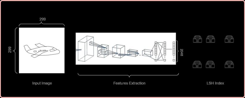
4.3   Best Model Choice
After training, we test each model in terms of mean average precision mAP. Specifically, for
each of the 250 classes in the sketches dataset, we hold out 20 out of 80 class samples as test
set so as to use one image from the test set as query object. The mAP is computed on a set of
250 queries, one per class, using cosine similarity as ranking measure. In the graph below we
report model test mAP (on the x axis) as a function of model complexity in terms of number
of parameters (on the y axis).

                               Figure 4: Test mAP vs Model Complexity

   As you can notice the best performing model in terms of mAP, which is the best metric for
CBIR systems evaluation, is the Model number 4. Notice that, in this phase of the project, all
models have been tested by performing sequential scan of the deep features so as to avoid the
additional bias introduced by the LSH index approximation.

University of Pisa. Sketches image analysis: Web image search engine using
                                             LSH index and DNN InceptionV3

5     LSH parameters tuning
In LSH it is extremely important to properly tune the parameters in order to discover the best
configuration in terms of trade-off between retrieval accuracy and efficiency: while the retrieval
efficiency of the system improves the accuracy decreases accordingly since the approximation
is tougher. As system retrieval accuracy metric we adopt test mean average precision mAP (the
same used for choosing the best network architecture). As far as system retrieval efficiency
is concerned, we use Improvement In Efficiency IE which is a metric computed as the ratio
between the query cost without using the index (sequential scan of deep features) and the query
cost when using LSH index. The cost is measured in terms of number of distance computations
needed to answer a query.
     LSH index needs to be properly tuned in both the real valued and binary cases: the optimal
choice best suiting our system for the pair of parameters (L, K) needs to be investigated.
Increasing the number of projections axis (K, number of hash functions h) has the effect
of better separating dissimilar objects: the larger K the lower the probability of having two
objects falling within the same bucket. Conversely, fixed K, if we increase L, the number of g
hash functions, we increase the collision probability. We carry out several tests varying each
time L and/or k.
     Moreover, in each test, beside computing mAP and IE, we compute some useful statistics
in order to derive better insights on the impact of LSH parameters on the system. Specifically,
we measured:

    – Average Bucket Purity. This is a pure number whose purpose is to provide a measure of
     “bucket purity”: the larger is the number of samples belonging to the majority class within
      the bucket with respect to the total number of elements being in the bucket, the purest the
      bucket is. The average bucket purity is computed as the average of the ratios between the
      number of elements in the majority class and the total number of elements in each bucket.
    – Standard Deviation of Average Bucket Purity. This is the standard deviation of the
      average bucket purity distribution.
    – Number of Buckets. This is simply the total number of distinct buckets making up the
      index.
    – Number of Items. This is the total number of objects contained within the index.
    – Average number of elements per bucket.
    – Standard Deviation of Average number of elements per bucket.

    In the following table we show results obtained in correspondence of each real valued LSH
index parameters configuration tried.

    Observations. Analyzing the numbers reported in the table you can notice that increasing
the value of k, the number of hash functions h, while the Improvement in Efficiency IE
improves of three orders of magnitude (from 0.46 for k = 1 up to 4, 000 for k = 5), the mAP
of the system mutates in the opposite way (from the best value 37% for k = 1 down to 0.02 for
k = 5). Moreover, as k increases, the number of buckets increases by two orders of magnitude
(from 150 buckets when k=1 up to 24, 636 buckets when k = 5) and the Average Bucket Purity
increases (from 52% when k = 1 up to k = 5 when k = 5) accordingly. These experimental
results are aligned with what one would expect: increasing the number of projection axis, the

University of Pisa. Sketches image analysis: Web image search engine using
                                           LSH index and DNN InceptionV3

probability that any two objects fall within different buckets increases. Hence, the number
of buckets increases, the average number of items within each bucket decreases and as a
consequence the Average Bucket Purity increases: it is as if you were implementing a more
fine-grained clustering on data, thus having an higher probability of having samples belonging
to the same class within each cluster.
    As far as parameter L is concerned, the number of g hash functions, which also corresponds
to the number of index replicas you have, fixed K, as L increases, while mAP increases, IE
decreases (indeed the larger is L , the larger is the total number of items and the larger is
the number of distance computations needed to answer to a query). Furthermore, being L
the number of index replicas, if the index is held in main memory as it is the case in our
implementation, it cannot exceed a certain value depending on the size of the data to be
indexed and the amount of main memory available for the system.
    As highlighted in green within the table, in our specific use case, the parameters configura-
tion yielding the best trade-off between system efficiency and accuracy is L = 7 and K = 2.
With this configuration we obtain an IE of 4 meaning that we have an improvement in retrieval
cost by a factor of 4 and at the same time we do not loose too much in terms of mAP (26%
against 40% obtained when performing sequential scan without index).
    In the following table we show results obtained in correspondence of each binary valued
LSH index parameters configuration tried.

    Observations. As far as L and K parameters is concerned, similar observations as the
real valued LSH index case. It is interesting to compare the best real valued LSH index result
against the best binary valued LSH index in order to highlight the differences. The two results
are reported in the table below.
    As you can notice, in the Binary LSH case, we reach better performances both in terms of
system efficiency with an IE of 8.2 against the 3.9 of the Real LSH and in terms of system
accuracy with a mAP of 32% against the 26% of the Real LSH. It is interesting to observe
that the number of buckets in the binary case is much smaller (by an order of magnitude)
than the real case (192 against 2319). Additionally, it can be noticed that the Average Bucket
Purity value is smaller in the Real LSH case, indeed the average number of bucket items the
buckets is about six times larger. Hence, in the binary case we have much less buckets each
containing a larger number of objects, belonging to more classes: you would expect to obtain
a worse mAP value but it is not the case, since, as we will point out in the next paragraph, in
the Sketches dataset there are often very similar samples belonging to different classes.

University of Pisa. Sketches image analysis: Web image search engine using
                                             LSH index and DNN InceptionV3

6     Class by class analysis
During the development of the project, when testing the system with a set of random queries,
we noticed that the mAP score obtained from time to time varied largely: when using a sample
belonging to certain classes as query the mAP score obtained was quite good while it was
very bad in correspondence of some other samples belonging to other classes. Therefore, we
thought of investigating in order to gain insights on specific classes by carrying out a class by
class analysis.
    Specifically, for each individual class in the Sketches dataset, we computed both the mAP
and the CNN model Recall in such a way to be able to carry out a correlation analysis between
the two.

     As far as the class mAP computation is concerned, we proceeded as follows.

    Algorithm 1: Class by class analysis process
        For each element class (ci ) in array class (C);
        foreach ci ∈ C do
            For each class sample (sj ) in array element class (ci );
            foreach sj ∈ ci do
                execute query(sj ) ;
                AP ← compute AP(sj ) ;
            mAP ← compute mAP(ci ) ;
            max ← compute max(AP, ci ) ;
            min ← compute min(AP, ci ) ;
            range ← compute range(AP, ci ) ;
            std ← compute std(AP, ci ) ;
            show best sketch(ci ) ;
            show worst sketch(ci ) ;

    For each class, iteratively query the Sketches dataset, using each time one object the class
as query to retrieve all the others. Compute the Average Precision for each query. Then, for
each class, compute the class mAP, the minimum and maximum mAP values, the difference
between the maximum mAP and the minimum mAP and the mAP standard deviation. Finally,
return the Sketch in correspondence of which the maximum mAP value has been obtained and
the one for which the minimum mAP has been obtained.

    As output from this algorithm we obtained, for each class, a dictionary as the one that
follows.

                               Figure 5: Output Class by Class algorithm

University of Pisa. Sketches image analysis: Web image search engine using
                                           LSH index and DNN InceptionV3

    Beside this we computed the CNN model Recall score for each of the 250 Sketches dataset
classes: what is the percentage of samples belonging to each class correctly recognized by our
DL model. Then we carried out a correlation analysis between model class Recall and class
mAP, the scatter plot resulting is reported below.

                                   Figure 6: Recall and mAP by class

    We obtained a correlation coefficient of 0.79 highlighting, as expected, a significant
positive correlation between class Recall and class mAP.
    We conclude by reporting two examples: a first one showing data obtained for one of the
well-recognized classes and a second one showing data obtained in correspondence of one of
the bad-recognized classes.
    Well-recognized class example:

                               Figure 7: Well recognized class example

   As it can be noticed, it this case the system provides the user with mostly relevant results
expect when the input sketch is particularly badly drawn. Indeed, boomerang sketches are very
similar one with respect to the others and the class Recall value is 90

University of Pisa. Sketches image analysis: Web image search engine using
                                           LSH index and DNN InceptionV3

                               Figure 8: Bad recognized class example

    The Dog class provides interesting results: if you look at the best and the worst sketch
according to the Average Precision value obtained, these are reversed with respect to the
judgment you would state according to your sense of aesthetics. This is due to the fact that, if
you observe the other samples from the Dog class, these are all quite badly drawn, thus the
only good looking dog sketch is an outlier yielding different features. Additionally, the class
samples are all quite different one from the others, causing the low Recall and mAP values of
respectively 30% and 10%.

7   Conclusion and Future Works
Combining deep features extraction, exploiting transfer learning, and the approximate simi-
larity search method LSH, we succeeded in building a CBIR system which is both efficient
and accurate. Other indexing approaches could have been used for this purpose, e.g., scalar
quantization [5]. We developed a web application on top of the system so as to provide users
with a friendly graphical interface through which they can draw sketches in input as queries.
Most of the time the system provides fast and relevant answers to user needs.
     Video search engines, such as [2, 3, 4] developed by the AIMH Lab [1], would benefit
from sketches image analysis. Integrating the propose approach with them is a future work.

Acknowledgments
This work is the result of the student project made in the course “Multimedia Information
Retrieval and Computer Vision” (Prof. Giuseppe Amato, Claudio Gennaro and Fabrizio Falchi)
for the Master Degree in ”Artificial Intelligence and Data Engineering” of the University of
Pisa.

University of Pisa. Sketches image analysis: Web image search engine using
                                            LSH index and DNN InceptionV3

References
1. N. Aloia, A. Giuseppe, B. Valentina, B. Filippo, B. Paolo, C. Fabio, C. Vittore, C. Luca, C. Cesare,
C. Silvia, E. Andrea, F. Fabrizio, G. Claudio, L. Gabriele, M. F. Valerio, M. Carlo, M. Nicola,
M. Daniele, M. Alessio, M. Alejandro, N. Alessandro, P. Aandrea, P. Nicolò, R. Fauto, S. Pasquale,
S. Fabrizio, T. Costantino, T. Luca, V. Lucia, and V. Claudio. Aimh research activities 2020. Technical
Report 413891, Consiglio Nazionale delle Ricerche, 2020.
2. G. Amato, P. Bolettieri, F. Carrara, F. Debole, F. Falchi, C. Gennaro, L. Vadicamo, and C. Vairo.
Visione at vbs2019. In I. Kompatsiaris, B. Huet, V. Mezaris, C. Gurrin, W.-H. Cheng, and S. Vrochidis,
editors, MultiMedia Modeling, pages 591–596, Cham, 2019. Springer International Publishing.
3. G. Amato, P. Bolettieri, F. Carrara, F. Debole, F. Falchi, C. Gennaro, L. Vadicamo, and C. Vairo.
The visione video search system: Exploiting off-the-shelf text search engines for large-scale video
retrieval. Journal of Imaging, 7(5), 2021.
4. G. Amato, P. Bolettieri, F. Falchi, C. Gennaro, N. Messina, L. Vadicamo, and C. Vairo. Visione
at video browser showdown 2021. In J. Lokoč, T. Skopal, K. Schoeffmann, V. Mezaris, X. Li,
S. Vrochidis, and I. Patras, editors, MultiMedia Modeling, pages 473–478, Cham, 2021. Springer
International Publishing.
5. G. Amato, F. Carrara, F. Falchi, C. Gennaro, and L. Vadicamo. Large-scale instance-level image
retrieval. Information Processing & Management, 57(6):102100, 2020.
6. M. S. Charikar. Similarity estimation techniques from rounding algorithms. In Proceedings of the
Thiry-Fourth Annual ACM Symposium on Theory of Computing, STOC ’02, page 380–388, New York,
NY, USA, 2002. Association for Computing Machinery.
7. M. Datar, N. Immorlica, P. Indyk, and V. S. Mirrokni. Locality-sensitive hashing scheme based on p-
stable distributions. In Proceedings of the Twentieth Annual Symposium on Computational Geometry,
SCG ’04, page 253–262, New York, NY, USA, 2004. Association for Computing Machinery.
8. A. Gionis, P. Indyk, and R. Motwani. Similarity search in high dimensions via hashing. In
Proceedings of the 25th International Conference on Very Large Data Bases, VLDB ’99, page 518–529,
San Francisco, CA, USA, 1999. Morgan Kaufmann Publishers Inc.
9. M. J. Huiskes and M. S. Lew. The mir flickr retrieval evaluation. In Proceedings of the 1st ACM
International Conference on Multimedia Information Retrieval, MIR ’08, page 39–43, New York, NY,
USA, 2008. Association for Computing Machinery.
10. P. Li and A. C. König. Theory and applications of b-bit minwise hashing. Communications of the
ACM, 54(8):101–109, 2011.
11. C. Szegedy, V. Vanhoucke, S. Ioffe, J. Shlens, and Z. Wojna. Rethinking the inception architecture
for computer vision. CoRR, abs/1512.00567, 2015.