Snow Cover Monitoring with MODIS Satellite Data in Alaska's National Parks, 2000-2015 - Natural Resource Report NPS/SWAN/NRR-2017/1566
←
→
Page content transcription
If your browser does not render page correctly, please read the page content below

National Park Service
U.S. Department of the Interior

Natural Resource Stewardship and Science

Snow Cover Monitoring with MODIS Satellite Data in
Alaska’s National Parks, 2000-2015
Natural Resource Report NPS/SWAN/NRR—2017/1566
ON THE COVER
This image is a natural color RGB from the MODIS sensor at 2017-04-13 22:35 UTC showing snow covered but cloud-free
conditions over most of Alaska
Image obtained from the Geographic Information Network of Alaska’s (GINA’s) Puffin imagery server
Snow Cover Monitoring with MODIS Satellite Data in
Alaska’s National Parks, 2000-2015
Natural Resource Report NPS/SWAN/NRR—2017/1566

Jessica E. Cherry,1 Jiang Zhu,1 Peter B. Kirchner,2

1
 The Geographic Information Network of Alaska
University of Alaska Fairbanks
111 WRRB
Fairbanks, AK 99775

2
 National Park Service
Southwest Alaska Network
240 West 5th Avenue
Anchorage, AK 99501

December 2017

U.S. Department of the Interior
National Park Service
Natural Resource Stewardship and Science
Fort Collins, Colorado
The National Park Service, Natural Resource Stewardship and Science office in Fort Collins,
Colorado, publishes a range of reports that address natural resource topics. These reports are of
interest and applicability to a broad audience in the National Park Service and others in natural
resource management, including scientists, conservation and environmental constituencies, and the
public.

The Natural Resource Report Series is used to disseminate comprehensive information and analysis
about natural resources and related topics concerning lands managed by the National Park Service.
The series supports the advancement of science, informed decision-making, and the achievement of
the National Park Service mission. The series also provides a forum for presenting more lengthy
results that may not be accepted by publications with page limitations.

All manuscripts in the series receive the appropriate level of peer review to ensure that the
information is scientifically credible, technically accurate, appropriately written for the intended
audience, and designed and published in a professional manner. This report received informal peer
review by subject-matter experts who were not directly involved in the collection, analysis, or
reporting of the data.

Views, statements, findings, conclusions, recommendations, and data in this report do not necessarily
reflect views and policies of the National Park Service, U.S. Department of the Interior. Mention of
trade names or commercial products does not constitute endorsement or recommendation for use by
the U.S. Government.

This report is available in digital format from Southwest Alaska Network website and the Natural
Resource Publications Management website. To receive this report in a format that is optimized to be
accessible using screen readers for the visually or cognitively impaired, please email irma@nps.gov.

Please cite this publication as:

Cherry, J. E., J. Zhu, and P. B. Kirchner. 2017. Snow cover monitoring with MODIS satellite data in
Alaska’s national parks, 2000-2015. Natural Resource Report NPS/SWAN/NRR—2017/1566.
National Park Service, Fort Collins, Colorado.

NPS 953/141364, December 2017
                                                  ii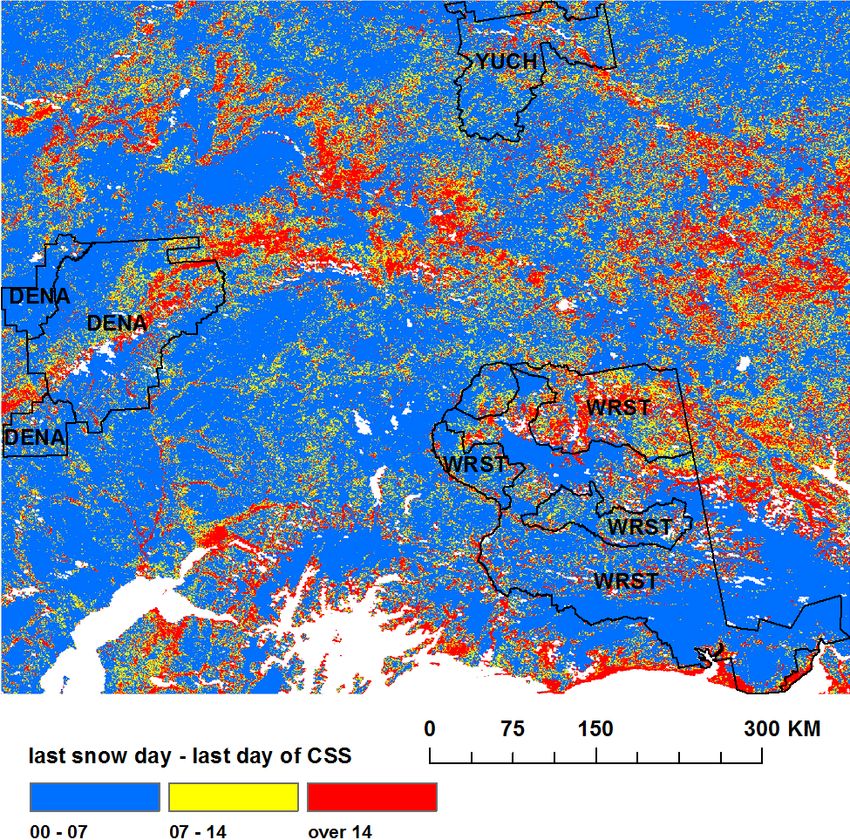
Contents
                                                                                                                                                     Page

Figures................................................................................................................................................... iv

Tables ..................................................................................................................................................viii

Abstract ................................................................................................................................................. ix

Acknowledgments.................................................................................................................................. x

List of Terms and Acronyms ................................................................................................................ xi

Introduction ............................................................................................................................................ 1

Study Areas and Methods ...................................................................................................................... 2

       State of Alaska as a Whole ............................................................................................................. 2

       ARCN ............................................................................................................................................. 5

       CAKN ............................................................................................................................................. 8

       SEAN............................................................................................................................................ 10

       SWAN .......................................................................................................................................... 13

       Image Processing .......................................................................................................................... 16

       Data Analysis ............................................................................................................................... 18

       Accuracy Assessment ................................................................................................................... 18

Results and Discussion ........................................................................................................................ 21

       Alaska and Neighboring Areas ..................................................................................................... 21

       ARCN ........................................................................................................................................... 32

       CAKN ........................................................................................................................................... 39

       SEAN............................................................................................................................................ 52

       SWAN .......................................................................................................................................... 65

Literature Cited .................................................................................................................................... 79

                                                                            iii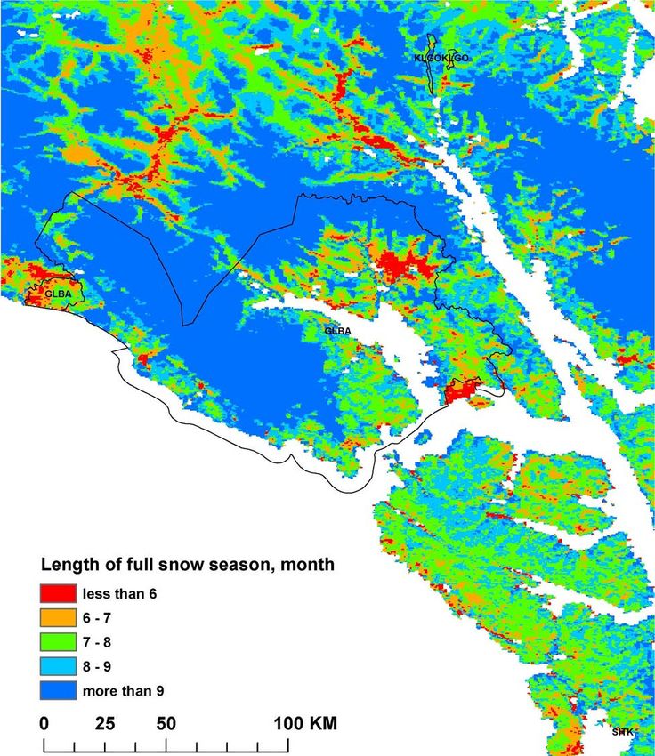
Figures
Page
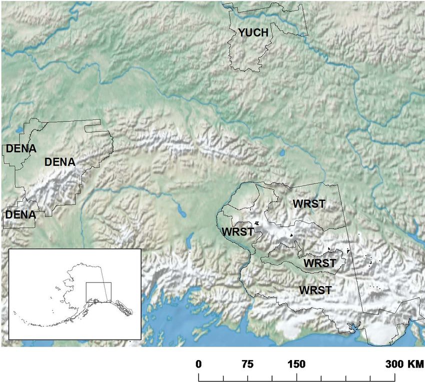
Figure 1. A map showing the locations of the NPS Networks and Units in Alaska ............................. 2
Figure 2. SNAP 2000-2009 Annual Average Temperature Climatology from CRU and
PRISM climate models, in degrees Celsius. .......................................................................................... 3
Figure 3. SNAP 2000-2009 Annual Average Precipitation Climatology from CRU and
PRISM climate models, in millimeters. ................................................................................................. 4
Figure 4. Average air temperatures at long-term stations near the Alaska Park Networks .................. 4
Figure 5. Average precipitation at long-term stations near the Alaska Park Networks ........................ 5
Figure 6. Average snowfall at long-term stations near the Alaska Park Networks .............................. 5
Figure 7. The Arctic Inventory and Monitoring Network (ARCN) Parks and Preserves. .................... 6
Figure 8. SNAP 2000-2009 Annual Average Surface Air Temperature Climatology from
CRU and PRISM in degrees Celsius...................................................................................................... 7
Figure 9. SNAP 2000-2009 Annual Average Precipitation Climatology from CRU and
PRISM.................................................................................................................................................... 7
Figure 10. The Central Alaska Inventory and Monitoring (CAKN) Parks and Preserves. ................... 8
Figure 11. SNAP 2000-2009 Annual Average Temperature Climatology from CRU and
PRISM.................................................................................................................................................... 9
Figure 12. SNAP 2000-2009 Annual Average Precipitation Climatology from CRU and
PRISM, 2x2 km. .................................................................................................................................. 10
Figure 13. The Southeast Alaska Inventory and Monitoring Network (SEAN) Parks and
Preserves. ............................................................................................................................................. 11
Figure 14. SNAP 2000-2009 Annual Average Temperature Climatology from CRU and
PRISM.................................................................................................................................................. 12
Figure 15. SNAP 2000-2009 Annual Average Precipitation Climatology from CRU and
PRISM.................................................................................................................................................. 13
Figure 16. The Southwest Alaska Inventory and Monitoring Network (SWAN) Parks and
Preserves. ............................................................................................................................................. 14
Figure 17. SNAP 2000-2009 Annual Average Temperature Climatology from CRU and
PRISM.................................................................................................................................................. 15
Figure 18. SNAP 2000-2009 Annual Average Precipitation Climatology from CRU and
PRISM.................................................................................................................................................. 16
iv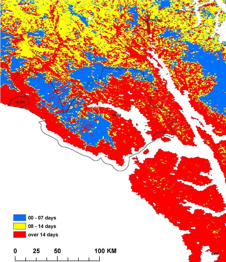
Figures (continued)
                                                                                                                                                      Page

Figure 19a-d. Boxplots summarizing bias (observed–predicted) for four MODIS-derived
snow season metrics: (A) First Snow Day, (B) CSS start (LCFD), (C) Last Snow Day and
(D) CSS end (LCLD), compared to three in situ weather station types............................................... 19

Figure 20. Landsat 1985 – 2011 last snow day, aggregated to 500m, vs 2001 – 2015
MODIS last snow day .......................................................................................................................... 20

Figure 21. Median first snow day for the years 2001-2015. ............................................................... 22

Figure 22. Median start of continuous snow season (CSS) for years 2001-2015. .............................. 23

Figure 23. Median last snow day for years 2001-2015. ...................................................................... 24

Figure 24. Median end of CSS for years 2001-2015. ......................................................................... 25

Figure 25. Difference in days between the median last snow day and the median end of
the CSS................................................................................................................................................. 26

Figure 26. Standard deviation in the end of CSS, 2001-2015. ............................................................ 27

Figure 27. Median length of the full snow season in Alaska. ............................................................. 28

Figure 28. Median length of the continuous snow season (CSS) in Alaska. ...................................... 29

Figure 29. Linear Correlation Coefficient (r) of length of CSS for 2001-2015 .................................. 30

Figure 30. Same as Figure 29 but for the end of CSS. ........................................................................ 31

Figure 31. Median first snow day for the years 2001-2015. ............................................................... 32

Figure 32. Median start of continuous snow season (CSS) for years 2001-2015. .............................. 33

Figure 33. Median last snow day for years 2001-2015. ...................................................................... 33

Figure 34. Median end of CSS for years 2001-2015. ......................................................................... 34

Figure 35. Difference in days between the median last snow day and the median end of
the CSS................................................................................................................................................. 34

Figure 36. Standard deviation in the end of CSS, 2001-2015. ............................................................ 35

Figure 37. Mean deviation from the typical (median) end of CSS by ARCN NPS unit by
year....................................................................................................................................................... 35

Figure 38. Median length of the full snow season in ARCN. ............................................................. 36

Figure 39. Median length of the continuous snow season (CSS) in ARCN. ...................................... 36

                                                                              v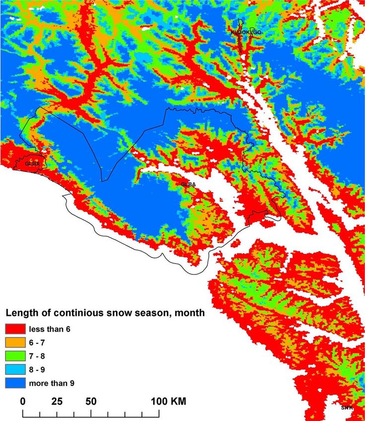
Figures (continued)
                                                                                                                                                   Page

Figure 40. Trends in the length of the CSS in ARCN ......................................................................... 37

Figure 41. Same as Figure 40 except for trends in the end of CSS in ARCN. ................................... 38

Figure 42. Mean of end days of continuous snow season at Kotzebue and surface air
temperature at Kotzebue airport ........................................................................................................... 38

Figure 43. Median first snow day for the years 2001-2015. ............................................................... 40

Figure 44. Median start of continuous snow season (CSS) for years 2001-2015. .............................. 41

Figure 45. Median last snow day for years 2001-2015. ...................................................................... 43

Figure 46. Median end of CSS for years 2001-2015. ......................................................................... 44

Figure 47. Difference in days between the median last snow day and the median end of
the CSS................................................................................................................................................. 45

Figure 48. Standard deviation in the end of CSS, 2001-2015. ............................................................ 46

Figure 49. Mean deviation from the typical (median) end of CSS by CAKN unit by year. ............... 47

Figure 50. Median length of the full snow season in CAKN. ............................................................. 48

Figure 51. Median length of the continuous snow season (CSS) in CAKN. ...................................... 49

Figure 52. Trends in the length of the CSS in CAKN ........................................................................ 50

Figure 53. The same as for Figure 52, but for the end of the CSS. ..................................................... 51

Figure 54. Mean of end days of continuous snow season at Talkeenta and surface air
temperature at Talkeetna airport .......................................................................................................... 52

Figure 55. Median first snow day for the years 2001-2015. ............................................................... 54

Figure 56. Median start of the continuous snow season (CSS) for years 2001-2015. ........................ 55

Figure 57. Median last snow day for years 2001-2015. ...................................................................... 56

Figure 58. Median end of CSS for years 2001-2015. ......................................................................... 57

Figure 59. Difference in days between the median last snow day and the median end of
the CSS................................................................................................................................................. 58

Figure 60. Standard deviation in the end of CSS, 2001-2015. ............................................................ 59

Figure 61. Mean deviation from the typical (median) end of CSS by SEAN unit by year. ................ 60

Figure 62. Median length of the full snow season in SEAN. .............................................................. 61

                                                                            vi
Figures (continued)
                                                                                                                                                   Page

Figure 63. Median length of the continuous snow season (CSS) in SEAN. ....................................... 62

Figure 64. Trends in the length of the CSS in SEAN. Red pixels have a T-test statistic
less than -0.51 indicating a significant linear correlation of snow cover decreasing over
the period of record .............................................................................................................................. 63

Figure 65. As in Figure 64 but for end of CSS. .................................................................................. 64

Figure 66. Mean of end days of continuous snow season at Haines and surface air
temperature at Haines airport ............................................................................................................... 65

Figure 67. Median first snow day for the years 2001-2015. ............................................................... 66

Figure 68. Median start of continuous snow season (CSS) for years 2001-2015. .............................. 67

Figure 69. Median last snow day for years 2001-2015. ...................................................................... 69

Figure 70. Median end of CSS for years 2001-2015. ......................................................................... 70

Figure 71. Difference in days between the median last snow day and the median end of
the CSS................................................................................................................................................. 71

Figure 72. Standard deviation in the end of CSS, 2001-2015. ............................................................ 72

Figure 73. Mean deviation from the typical (median) end of CSS by SWAN unit by year. .............. 73

Figure 74. Median length of the full snow season in SWAN. ............................................................ 74

Figure 75. Median length of the continuous snow season (CSS) in SWAN....................................... 75

Figure 76. Mean of end days of continuous snow season at King Salmon and surface air
temperature at King Salmon airport ..................................................................................................... 76

Figure 77. Trends in the length of the CSS in SWAN. Red pixels have a T-test statistic
less than -0.51 indicating a significant linear correlation of snow cover decreasing over
the period of record .............................................................................................................................. 77

Figure 78. As in Figure 77 but for end of CSS. .................................................................................. 78

                                                                           vii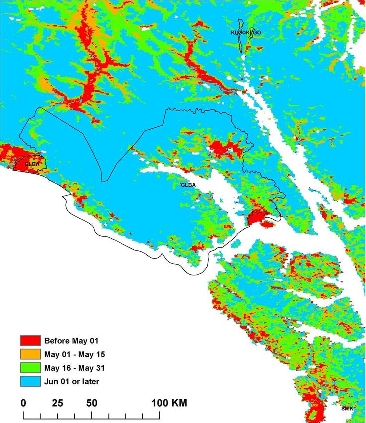
Tables
                                                                                                                                                   Page

Table 1. Snow Metrics Mean (Standard Deviation) Data in Alaska Summarized by
Elevation. ............................................................................................................................................. 31

Table 2. Snow Metrics Mean (Standard Deviation) Data in ARCN Summarized by
Elevation. ............................................................................................................................................. 39

Table 3. Snow Metrics Mean (Standard Deviation) Data in CAKN Summarized by
Elevation. ............................................................................................................................................. 42

Table 4. Snow Metrics Mean (Standard Deviation) Data in SEAN Summarized by
Elevation. ............................................................................................................................................. 53

Table 5. Snow Metrics Mean (Standard Deviation) Data in SWAN Summarized by
Elevation. ............................................................................................................................................. 68

                                                                           viii
Abstract
Snow cover has a profound effect on flora, fauna, and the physical environment of Alaska’s National
Parks and Preserves. The generation of the datasets presented here is motivated by questions about
potential changes in snow cover in recent decades. Geospatial time series and statistical analyses of
the first and last days of snow cover, the continuous snow season (CSS), and their trends are
performed with a snow cover extent product derived from the Moderate Resolution Imaging
Spectroradiometer (MODIS) satellite sensor for the Alaska National Park Service Inventory and
Monitoring (I&M) Networks and the state as a whole (2001-2015).
The end of the CSS is a relatively robust measure of change in the spring snowpack, driven by
changes in temperature and precipitation. Changes in the length of the CSS are more uncertain
because cloud cover in the autumn, in particular, can lead to errors in the estimates of the start of the
snow season. Results of parametric and non-parametric statistical tests are similar. CSS trends at
various stations seem to track with temperature trends during the melt season, but are not statistically
significant. Precipitation factors are hard to discern due to the difficult nature of precipitation
measurement in the Arctic.
The Northwest Alaskan Arctic stands out as the biggest region where the length of the CSS has
decreased significantly and the end of the CSS is coming a week or two earlier in 2015 than it did in
2001. Upstream and downstream of Northwest Alaska—Eastern Siberia and the Upper Yukon basin
in Southern Yukon Territory and Northern British Columbia, Canada—show the opposite trends.
ixAcknowledgments
The authors wish to acknowledge Tom Heinrichs, Dayne Broderson, and Colleen Morey of the
Geographic Information Network of Alaska (GINA), for their help in administrating this research.
David K. Swanson, of the National Park Service (NPS), generously provided a template and
guidance for this effort. Parker Martyn, Amy Miller, and Chuck Lindsay, all of the NPS, provided
helpful comments on this manuscript during its development. The GINA authors acknowledge
financial support from NPS under agency award number P13AC00836.
xList of Terms and Acronyms
ALAG: Alagnak Wild River
ANIA: Aniakchak National Monument and Preserve
ARCN: Arctic Inventory and Monitoring Network
BELA: Bering Land Bridge National Park
CAKN: Central Alaska Inventory and Monitoring Network
CAKR: Cape Krusenstern National Monument
DENA: Denali National Park
GAAR: Gates of the Arctic National Park and Preserve
GLBA: Glacier Bay National Park and Preserve
KATM: Katmai National Park and Preserve
KEFJ: Kenai Fjords National Park
KLGO: Klondike Gold Rush National Historic Park
KOVA: Kobuk Valley National Park
LACL: Lake Clark National Park and Preserve
NOAT: Noatak National Preserve
SEAN: Southeast Alaska Inventory and Monitoring Network
SITK: Sitka National Historic Park
SWAN: Southwest Alaska Inventory and Monitoring Network
WRST: Wrangell-St. Elias National Park
YUCH: Yukon Charley National Preserve
xiIntroduction
Snow is a dominant feature of the Alaskan landscape throughout a typical cold season. It has a
profound effect on the regional climate via its albedo, which is the fraction of incoming solar
radiation that is reflected back into the atmosphere. When new snow is present, approximately 80-
95% of incoming solar radiation is reflected directly back into the atmosphere (Armstrong and
Brown 2008). In the absence of low clouds, this leads to very stable cold air masses and atmospheric
temperature inversions. The persistent winter high pressure over Alaska’s Interior is a dynamical
impact of the surface energy budget over a large continental land mass. In the absence of snow, the
land surface absorbs 70-90% of the incoming solar radiation and re-radiates this energy in the long-
wave part of the electromagnetic spectrum, warming the overlying atmosphere (King et al. 2008).
Climate change may lead to a variety of hydroclimate shifts in Alaska. In southern Alaska, where
atmospheric moisture is plentiful, a warming atmosphere may drive a phase change in precipitation,
causing more rain to fall in lieu of snow, particularly at high altitudes. In the Interior and Northern
parts of the state, which have had very dry climates in modern times, climate change may bring
warmer and moister air, leading to an increase in snowfall. In Far Northern coastal regions, changes
in snow are thought to be impacted by changes in sea ice cover, via a “lake effect” snow mechanism
of open water during the cold season. However, these types of hydroclimate changes have been
difficult to detect with a very sparse station network with strong spatial and temporal variability
(McAfee et al. 2013).
The National Park Service (NPS) is interested in monitoring changes in snow cover because of the
strong impact it has on landscape ecology, the evolution of permafrost, and the animals whose
habitats and food sources depend on the presence or absence of snow, as well as its properties such as
density and hardness.
The challenge of monitoring snow is that it is difficult or labor intensive to measure snow falling or
resting on the land surface, and meaningful sampling requires capturing its spatial distribution.
Precipitation gauges have wind-induced under-catch of as much as 100% in high latitudes (Goodison
et al. 1998). Snow depth on the ground is currently measured by a manual observer (typically along a
transect) or by autonomous instrumentation that has a limited ability to sample the variability of
snow depth over landscapes (Ryan et al. 2008). All of these methods measure relatively small areas
and rarely capture the spatial variability of snow distribution across the landscape. Another challenge
to snow measurement in the high latitudes is snow redistribution by winds. There are no wide-scale
observational networks that specifically measure snow redistribution by wind in Alaska.
These difficulties with ground-based measurement of snow make remote sensing of snow cover
appealing as a tool for monitoring change. Even at moderate resolution (500 m pixels), the ability to
detect variability over the landscape, and statewide (or global) coverage enable a far bigger picture of
the extent of observed changes.
1Study Areas and Methods
This method focused on analysis of four different NPS Inventory and Monitoring Networks in
Alaska, as well as the state of Alaska as a whole (Figure 1). First, the Alaska region and each study
area will be described, then the image processing and the data analysis will be explained in the
following subsections. The methods, images, analysis, and accuracy assessment of these data are
further described in Swanson (2014) and Lindsay et.al. (2015). Data for each metric may be accessed
from the Geographic Information Network of Alaska at:
http://gina.alaska.edu/projects/modis-derived-snow-metrics
Figure 1. A map showing the locations of the NPS Networks and Units in Alaska. Sites of long-term
weather observations from the National Weather Service are marked and labeled.
State of Alaska as a Whole
Alaska’s existing NPS units are found in 10 of the state’s 13 regional climate divisions as described
by Bieniek et al. (2012). To provide a regional context with respect to park units, the MODIS-derived
snow cover statistics will be analyzed first for the Alaska region and then the four National Park
Service Inventory and Monitoring Networks. The climate throughout Alaska varies much like the
NPS units within the state, however the North Slope—the flat coastal plain north of the Brooks
Range—is further north and experiences a somewhat colder and drier climate than those represented
in ACRN (Figures 2 and 3). The geographic variability of climate is exemplified by the temperature
2and snowfall climographs from the National Weather Service long term monitoring stations (Figures
4-6).
Figure 2. SNAP 2000-2009 Annual Average Temperature Climatology from CRU and PRISM climate
models, in degrees Celsius.
3Figure 3. SNAP 2000-2009 Annual Average Precipitation Climatology from CRU and PRISM climate
models, in millimeters.
Figure 4. Average air temperatures at long-term stations near the Alaska Park Networks. Data are from
the National Climatic Data Center (NCDC) Global Historical Climate Network (GHCN) Normals (1981-
2010) product.
4Figure 5. Average precipitation at long-term stations near the Alaska Park Networks. Data are from the
NCDC GHCN Normals (1981-2010) product.
Figure 6. Average snowfall at long-term stations near the Alaska Park Networks. Data are from the
NCDC GHCN Normals (1981-2010) product.
ARCN
Alaska is home to four different Inventory and Monitoring Networks of the National Park Service
(Figure 1). The most northern and therefore coldest of these regional networks is the Arctic Inventory
and Monitoring Network (ARCN, Figure 7). Within this network are five NPS units that vary
considerably in their geography and climate. The Bering Land Bridge National Park (BELA) covers
the northern part of the Seward Peninsula and, along with the Cape Krusenstern National Monument
(CAKR) on the Northwestern coast, experience lowland, maritime climates in summer and quasi-
5continental climates when the Chukchi is ice covered. To the East, the Noatak National Preserve
(NOAT), the Kobuk Valley National Park and Preserve (KOVA), and the Gates of the Arctic
National Park and Preserve (GAAR) experience cold, continental climates, and also have dramatic,
varying terrain ranging from sand dunes near sea level to nearly 8000 feet (~2400 m). Typical daily
average air temperatures in this region creep above 0 °C in mid-May and drop back below 0 °C in
late September (Figure 4).
Figure 7. The Arctic Inventory and Monitoring Network (ARCN) Parks and Preserves.
These air temperatures vary spatially according to elevation and distance from the ocean from -2 °C
to -12 °C annual average surface air temperature (University of Alaska Fairbanks Scenarios Network
for Alaska Planning, Climate Research Unit, 2x2 km products, SNAP, 2016, Figure 8). Precipitation
is low throughout the year (Figure 5). Late 20th century climatologies of estimated cold season
precipitation (October-April, Climate Research Unit, 2x2 km, SNAP, 2016, Figure 9) show spatial
variability ranging from a cumulative 100-150 mm of precipitation in the BELA lowlands to 250-300
mm in GAAR.
6Figure 8. SNAP 2000-2009 Annual Average Surface Air Temperature Climatology from CRU and PRISM
in degrees Celsius.
Figure 9. SNAP 2000-2009 Annual Average Precipitation Climatology from CRU and PRISM. Units are in
mm.
7CAKN
The Central Alaska Inventory and Monitoring network (CAKN) encompasses three units ranging
from the Interior to South Central Alaska (Figure 10). The Yukon Charley National Preserve
(YUCH) is the coldest and most continental, as well as the furthest north of these units. YUCH
includes vast flat wetlands, as well as higher, more complex terrain. Denali National Park (DENA) is
the unit furthest to the west in this network and includes North America’s highest mountain as well
as other high terrain. Finally, Wrangell-St. Elias National Park (WRST), in South Central Alaska, is
America’s largest national park and encompasses terrain from coastlines to rugged mountains and
intermountain areas. Topography in CAKN ranges from sea level in Icy Bay to Mount Denali more
than 20,300 feet (6187 m).
Figure 10. The Central Alaska Inventory and Monitoring (CAKN) Parks and Preserves.
Long-term weather stations to the east of DENA and northwest of WRST show temperatures of a
continental climate—warm in summer and very cold in winter, however precipitation in these units is
8impacted by storms coming from the Gulf of Alaska, year-round (Figures 4 and 5). Fewer long-term,
instrumental records of temperature and precipitation exist in YUCH, but modeled products show a
strongly continental and dry climate (Figures 11 and 12).
Figure 11. SNAP 2000-2009 Annual Average Temperature Climatology from CRU and PRISM. Units are
in degrees Celsius.
9Figure 12. SNAP 2000-2009 Annual Average Precipitation Climatology from CRU and PRISM, 2x2 km.
Units are in mm.
SEAN
The Southeast Alaska Inventory and Monitoring network (SEAN) includes three units: the large
Glacier Bay National Park and Preserve (GLBA) along the coastal fjords, the tiny Klondike Gold
Rush National Historic Park (KLGO) in and nearby the city of Skagway, and the even smaller Sitka
National Historic Park (SITK), in the city of Sitka (Figure 13). All three units are on or near the
jagged coastline of Southeast Alaska, but they experience microclimates based on their topography,
distance and orientation from the open ocean (Figure 14). Summers in SEAN are cooler than in
CAKN but the winters are much warmer (Figure 4). Higher elevations in this region (which rise up to
~15,500 feet or ~4724 m) will maintain a continuous snowpack (and form glaciers in places), but at
10sea level the climate is relatively warm in winter; snow falls only intermittently and melts quickly.
Total precipitation in Southeast, however, is heavy, leading to its characterization as a temperate
rainforest (Figure 15).
Figure 13. The Southeast Alaska Inventory and Monitoring Network (SEAN) Parks and Preserves.
11Figure 14. SNAP 2000-2009 Annual Average Temperature Climatology from CRU and PRISM. Units are
degrees Celsius.
12Figure 15. SNAP 2000-2009 Annual Average Precipitation Climatology from CRU and PRISM. Units are
in mm.
SWAN
The Southwest Alaska Inventory and Monitoring Network (SWAN) has five units in Southcentral
and Southwest Alaska. From east to west, these are the Kenai Fjords National Park (KEFJ), on the
Kenai Peninsula, the Lake Clark National Park and Preserve (LACL), Katmai National Park and
Preserve (KATM), the Alagnak Wild River (ALAG), and the Aniakchak National Monument and
13Preserve (ANIA, Figure 16). All of these units have mountainous terrain (up to ~10,200 feet or 3,109
m), and sit on or near the coast of a peninsula, except for LACL on ‘mainland’ Alaska. The long-
term climate record at King Salmon shows average monthly air temperatures similar to Haines and
Talkeetna (Figures 4 and 17), but with much less winter precipitation than Haines and much less
snowfall than either Haines or Talkeetna (Figures 5 and 18).
Figure 16. The Southwest Alaska Inventory and Monitoring Network (SWAN) Parks and Preserves.
14Figure 17. SNAP 2000-2009 Annual Average Temperature Climatology from CRU and PRISM. Units are
degrees Celsius.
15Figure 18. SNAP 2000-2009 Annual Average Precipitation Climatology from CRU and PRISM. Units are
mm.
Image Processing
The image analysis was identical to that described in Swanson (2014) except that the end date was
extended through 2015. The remainder of this subsection is reproduced verbatim from Swanson
(2014):
16The MODIS Terra Snow Cover Daily L3 Global 500m Grid data (MOD10A1; NASA 2013)
from the National Snow and Ice Data center (NSIDC: http://nsidc.org/data/modis/) were
used to determine the snow season. The MODIS Terra satellite gathers multispectral data
daily at 10:30 AM local time. Data were available from this satellite from the fall of 2000
through the spring of 2013 at the time of writing. Each pixel was screened for clouds by
NSDIC using the MODIS cloud mask product MOD35_L2 (http://modis-
atmos.gsfc.nasa.gov/MOD35_L2/index.html; Ackerman et al. 2010). In cloud-free pixels,
snow cover (snow present or not present), snow albedo (the percentage of solar radiation
reflected), and fractional snow cover (estimated snow cover in percent) were mapped by the
NSIDC using a snow mapping algorithm based on the Normalized Difference Snow Index
(NDSI) and other criteria (Hall et al. 2006, Riggs et al. 2006). The snow cover
(presence/absence) value was derived from threshold tests applied to the NDSI and other
satellite measurements, while the fractional (percent) snow cover value was computed using
the regression relationship with NDSI developed by Salomonson and Appel (2004).
Determination of the start and end of the snow season is complicated by clouds and by the
fact the snow cover in a season may be interrupted by snow-free periods. Additional
processing of the daily NSIDC snow product, to interpolate across cloudy periods and detect
the start and end of snow cover periods of different lengths, was performed by the
Geographic Information Network of Alaska (GINA) at the University of Alaska, Fairbanks
(see http://www.gina.alaska.edu/projects/modis- derived-snow-metrics). The GINA snow
metrics algorithm involved repeated passes through the daily time-series data for each pixel,
forward and backward in time within each snow year. (A snow year was defined as August 1
to July 31). Pixels were classified as “snow covered” if they had >50% fractional snow
cover and albedo >30% on the NSIDC raster. First, a spatial filter removed isolated single
pixels of snow, no-snow, or cloud by assigning to the pixel the majority value of its 4 nearest
neighbors, if 3 or 4 of them were the same. Next, the value of “snow” or “no-snow” was
interpolated across all single-day cloudy periods bounded on both sides by the same class.
Then “snow” and “no- snow” classes were interpolated through longer cloudy periods, but
the routine differed depending on the time of year. The snow class was interpolated back in
time through cloudy periods in the winter and spring, while the no-snow class was
interpolated forward in time through cloudy periods in the fall. The very first and last snow
days (the “full snow season”) in the snow year were then located. The algorithm also
scanned for periods of continuous snow cover more than 2 weeks long with 2 or fewer days
of no-snow. The start and end of the longest of these continuous snow periods were
determined and the longest one was selected (the “continuous snow season”, CSS). For more
details of the algorithm used to derive the snow cover metrics, see Zhu and Lindsay (2013).
The following metrics from this processing were used in this report:
• First snow day – the first day of snow recorded in the snow year (i.e. after August 1).
This day can be followed by snow free periods before the start of CSS (below).
17• Last snow day – the last day of snow recorded prior to the end of the snow year (July 31).
Snow-free periods can separate the last snow day from the end of CSS (below).
• Start of CSS – the first day (in the fall) of the longest continuous snow season
• End of CSS – the last day (in the spring) of the longest continuous snow season
Terrain shadows as a function of sun elevation above the horizon were computed using the
ArcGIS “Hillshade” geoprocessing tool
(http://resources.arcgis.com/en/help/main/10.2/index.html#//009z000000v0000000)
assuming a sun azimuth of 157.5° (corresponding to 10:30 AM local time, the time of the
MODIS satellite pass). The formulas for computing the sun’s elevation above the horizon
through the year were taken from NOAA (2013).
Data Analysis
As in Swanson (2014), the medians of all 15 years of data were computed for the four metrics
analyzed here (first snow day, last snow day, start of CSS, end of CSS). The median is less affected
by anomalous values than the mean. Errors in the estimation of snow onset are introduced by low sun
angles, cloudiness, and terrain shadows. Because clear weather is more common in Alaska during the
snowmelt than snow onset, estimating the end of the snow season and the CSS is less prone to error
than estimating the start of the snow season.
To test for long-term trends in the timing of snow cover loss, least-squares linear regressions were
computed for the length of and end of CSS vs. year for each individual pixel, and tested for
significance with both a Student’s T-test (Snedecor and Cochrane 1989) and the Mann-Kendall trend
test (Mann 1945; Kendall 1975). Of these, the end of CSS results are likely to be the more robust
results because of the uncertainty in seasonal start time described above (and in Swanson 2014) and
the Mann-Kendall results may be more robust because they do not require normally distributed data.
Accuracy Assessment
A full accuracy assessment of the first snow day, last snow day, start of CSS and end of CSS, within
the context of snow classifications and in-situ observations, are fully described in Lindsay et al.
(2015). The following is a summary of those findings; for further information please see Lindsay et
al. (2015) and its supplements.
A comparison of MODIS-derived snow onset dates with in situ observations for locations stratified
by snow class was used to assess the accuracy of these data. Four snow classes: Tundra, Tiaga,
Maritime and Alpine as defined by Sturm et al. (1995) were combined into two groups
(Tundra/Tiaga, Maritime/Alpine) and tested using high quality snow cover observations from 244
stations in the SNOTEL, 1st Order climate stations and the Global Historic Climate Networks.
The results of this accuracy assessment showed first snow day were consistently earlier than those
measured at the stations and later for the last snow day (Figures 19a-d). In contrast the start of the
CSS was late for all classes and the end of the CSS was early. The modeled mean bias varied by type
of in-situ observation and snow class and ranged from −12.2 to 33.9 days. The lowest bias of −2.6 to
11 days was found at SNOTEL stations in Tundra/Taiga snow class and was highest in the coastal
18and Alpine classes. While this bias is a result of many factors the main contributors are the 50%
snow cover threshold of the algorithm that is sensitive to the heterogeneity and the variability of
snow cover and the presence of cloud cover, which tended to exacerbate both early and late bias thus
extending the snow season.
An investigation of MODIS-derived snow onset dates to the mean snow-free dates derived from
multiyear (1985–2011) 30 m Landsat data, aggregated to 500 m to match spatial resolutions was
conducted by Macander and Swingly (2017) and published as a USGS report. This study showed the
MODIS end of CSS to be 3.4 days earlier, on average, than snow-free dates with a mean absolute
difference between the two data sets of 4.2 days. The last snow day also showed good agreement
between the two multiyear snow persistence metrics, with a correlation of 0.79, a mean absolute error
of +/-4.5 days and a bias of -3.2 days, with the MODIS last snow day being earlier (Figure 20).
Figure 19a-d. Boxplots summarizing bias (observed–predicted) for four MODIS-derived snow season
metrics: (A) First Snow Day, (B) CSS start (LCFD), (C) Last Snow Day and (D) CSS end (LCLD),
compared to three in situ weather station types. The boxes depict the median, 1st and 3rd quartiles; the
whiskers depict the 10th and 90th percentiles; outliers are depicted by the open circles. Colors
correspond to combined snow class types. Figure reproduced from Lindsay et al., 2015.
19Figure 20. Landsat 1985 – 2011 last snow day, aggregated to 500m, vs 2001 – 2015 MODIS last snow
day. Figure reproduced from Macander and Swingley (2017).
20Results and Discussion
Variations in the timing and length of the snow seasons are likely linked to latitude, elevation, and
proximity to ocean and sea ice. Locally, the presence or absence of forest cover and aspect and
terrain, in combination with elevation, are key factors in smaller scale variation. Areas of high winds
and dry snow, especially in ARCN, are susceptible to snow redistribution by winds. Sturm et al.
(1995) characterize standard snow types by region in Alaska, which is helpful in thinking about the
factors behind variability in snow cover duration.
Alaska and Neighboring Areas
To provide a regionally comprehensive overview the figures and statistics are included (Figures 21-
30, Table 1). The results for the Alaska region are largely the sum of each regional network. The
Northwest Alaskan Arctic stands out as the biggest region where the length of the CSS has decreased
significantly and the end of the CSS is coming a week or two earlier in 2015 than it did in 2001. This
analysis does not go into detail to attribute the drivers of this change, but the fact that opposing trends
(more and later snow cover) can be seen clearly upstream in Eastern Siberia, and more sparsely in the
Upper Yukon basin (Figures 29 and 30) suggests that shifts in atmospheric circulation may be a
major driver at this timescale. This is consistent with findings in the literature (Cohen et al. 2012)
that suggest a radiative-dynamic coupling between snow cover and large-scale atmospheric
circulation in the Northern Hemisphere.
21Figure 21. Median first snow day for the years 2001-2015.
22Figure 22. Median start of continuous snow season (CSS) for years 2001-2015.
23Figure 23. Median last snow day for years 2001-2015.
24Figure 24. Median end of CSS for years 2001-2015.
25Figure 25. Difference in days between the median last snow day and the median end of the CSS.
26Figure 26. Standard deviation in the end of CSS, 2001-2015.
27Figure 27. Median length of the full snow season in Alaska.
28Figure 28. Median length of the continuous snow season (CSS) in Alaska.
29Figure 29. Linear Correlation Coefficient (r) of length of CSS for 2001-2015. Red pixels have a T-test
statistic less than -0.51 indicating a significant linear correlation of snow cover decreasing over the period
of record. Blue pixels have a T-test statistic greater than 0.51 indicating a significant linear correlation of
snow cover increase over the period of record. Green pixels show no significant trend according to a T-
test. The results from the Mann-Kendall test are very similar.
30Figure 30. Same as Figure 29 but for the end of CSS.
Table 1. Snow Metrics Mean (Standard Deviation) Data in Alaska Summarized by Elevation.
Snow Season 0-305 m 305-620 m 620-914 m 914-1219 m 1219-1524 m >1524 m
Metric 0-1000 ft 1000-2000 ft 2000-3000 ft 3000-4000 ft 4000-5000 ft >5000 ft Total
Median first 10/10(13) 10/02 (13) 09/28 (15) 09/20 (19) 09/11 (22) 08/23 (21) 10/02(18)
snow day
Median start of 10/27(20) 10/16(17) 10/10(17) 10/02(22) 09/21(26) 09/02(30) 10/17(24)
CSS
Median last 05/10(17) 05/16(15) 05/19(19) 05/28(25) 06/08(28) 07/01(28) 05/17(22)
snow day
Median end of 05/01(29) 05/10(19) 05/14(21) 05/23(27) 06/02(32) 06/24(33) 05/09(29)
CSS
Median length 216(26) 231(24) 240(30) 254(40) 274(47) 313(47) 231(38)
of full snow
season, days
Median length 186(44) 205(32) 217(34) 233(46) 254(56) 293(61) 204(50)
of CSS, days
31ARCN
In the Arctic Network, the median onset of the snow season and the CSS start earliest in the Brooks
Range with snowfall before September and continuous snow cover within the first two weeks of
September (Figures 31 and 32). The western-most areas, near the Chukchi Sea, see snowfall a good
six weeks later with continuous snow cover setting in about the same time. The areas in between see
snowfall in late September and continuous snow cover by early October. The end of the snow season
and the continuous snow season occur at about the same time in ARCN, with the earliest snowmelt in
the low lying areas (late April) and the latest at high elevations (after June), with coastal areas
melting out somewhere in between (Figures 33-35). The highest standard deviations in the end of the
CSS are in the highest parts of the Brooks Mountain Range, where snow redistribution by wind may
be a factor (Figure 36). A time series of standard deviations in the end of CSS shows a lot of
interannual variability in all the ARCN units (Figure 37). The longest snow seasons and CSS are in
the Brooks Range and other high elevations and the shortest are in the continental, lower lying areas
(Figures 38 and 39).
Figure 31. Median first snow day for the years 2001-2015.
32Figure 32. Median start of continuous snow season (CSS) for years 2001-2015.
Figure 33. Median last snow day for years 2001-2015.
33Figure 34. Median end of CSS for years 2001-2015.
Figure 35. Difference in days between the median last snow day and the median end of the CSS.
34Figure 36. Standard deviation in the end of CSS, 2001-2015.
Figure 37. Mean deviation from the typical (median) end of CSS by ARCN NPS unit by year.
35Figure 38. Median length of the full snow season in ARCN.
Figure 39. Median length of the continuous snow season (CSS) in ARCN.
36The statistical tests show that ARCN had the largest density of trends in the length and end of CSS
for the whole state, for 2001-2015, and where they are significant, these are almost exclusively
showing a shorter CSS and earlier end of CSS (Figures 40 and 41). The spatial pattern between these
two statistics varies slightly: the shorter CSS tends to be in the coastal and low-lying interior areas, as
well as the highest elevations, and the earlier end of CSS tends to be in the mid-elevation and the
mountainous areas (Figures 40, 41, and Table 2). The results of the T-test and the Mann-Kendall test
are very similar, so only the T-tests are shown here. Analysis of the surface air temperature at
Kotzebue shows no significant trend since 2001 (Figure 42). Likewise, the end of CSS in the 16
pixels surrounding Kotzebue shows no significant trend according to the T-test and the Mann-
Kendall test (Figure 42), but the two are inversely related: as the air temperatures increase in the
spring, the CSS ends earlier. The presence of snow also impacts overlying air temperatures, in turn.
However, these trends are not statistically significant over such a short period of record. McAfee et
al. (2013) suggest via both a literature search and an original analysis that annual and winter
precipitation at Kotzebue and Bettles have both likely increased since 1950 and 1980. The Alaska
Climate Research Center (ACRC 2016) show a significant winter and spring warming since 1949 at
Kotzebue and Bettles.
Figure 40. Trends in the length of the CSS in ARCN. Red pixels have a T-test statistic less than -0.51
indicating a significant linear correlation of snow cover decreasing over the period of record. Blue pixels
have a T-test statistic greater than 0.51 indicating a significant linear correlation of snow cover increase
over the period of record. Green pixels show no significant trend according to a T-test. The results from
the Mann-Kendall test are very similar.
37Figure 41. Same as Figure 40 except for trends in the end of CSS in ARCN.
Figure 42. Mean of end days of continuous snow season at Kotzebue and surface air temperature at
Kotzebue airport. Air temperature values are monthly averaged daily minimums. As temperatures go up,
CSS generally go down. Trends are not significant according to T-test and Mann-Kendall test.
38Table 2. Snow Metrics Mean (Standard Deviation) Data in ARCN Summarized by Elevation.
Snow Season 0-305 m 305-620 m 620-914 m 914-1219 m 1219-1524 m >1524 m
Metric 0-1000 ft 1000-2000 ft 2000-3000 ft 3000-4000 ft 4000-5000 ft >5000 ft Total
Median first
10/11(8) 10/01 (7) 09/27 (7) 09/21 (9) 09/13 (9) 09/05(10) 09/29(12)
snow day
Median start of
10/20(6) 10/09(6) 10/03(5) 09/28(5) 09/23(5) 09/17(7) 10/08(11)
CSS
Median last
05/17(7) 05/20(7) 05/20(8) 05/23(8) 05/28(9) 06/04(10) 05/21(8)
snow day
Median end of
05/16(6) 05/18(7) 05/17(8) 05/19(8) 05/22(10) 05/25(11) 05/18(8)
CSS
Median length
of full snow 222(14) 235(13) 241(14) 250(15) 260(15) 276(16) 238(20)
season, days
Median length
209(10) 222(11) 226(11) 232(11) 241(14) 251(16) 223(16)
of CSS, days
CAKN
In the Central Alaska Network, the median onset of the snow season and the CSS start earliest in the
Alaska Range, Chugach, and Wrangell Mountains with snowfall before September and continuous
snow cover within the first two weeks of September (Figures 43, 44, and Table 3). While some of
these areas contain glaciers and year-round snow, the snowline starts to progress down into the
foothills by early September. The YUCH flats see snow later, simply because the average elevation is
much lower throughout this unit. The end of the snow season and the continuous snow season
typically occur before May 1 throughout the low lying areas of CAKN, nearly a month later in the
foothills, with continuous snow cover in areas of the mountains with glaciers and permanent
snowfields (Figures 45 and 46). Figure 47 shows that the biggest difference between the end of the
snow season and the end of the CSS are in areas of moderate topography where it is cool enough for
late season snowfall. The highest standard deviations in the end of the CSS are also largely in the
areas of moderate topography (Figure 48), because much of the highest topography is glaciated. A
time series of standard deviations in the end of CSS shows high interannual variability in all the
CAKN units (Figure 49). Snow season length in CAKN closely follows topography with the low
lying river valleys having the shortest snow seasons (Figures 50 and 51).
39Figure 43. Median first snow day for the years 2001-2015.
40Figure 44. Median start of continuous snow season (CSS) for years 2001-2015.
41Table 3. Snow Metrics Mean (Standard Deviation) Data in CAKN Summarized by Elevation.
Snow Season 0-305 m 305-620 m 620-914 m 914-1219 m 1219-1524 m >1524 m
Metric 0-1000 ft 1000-2000 ft 2000-3000 ft 3000-4000 ft 4000-5000 ft >5000 ft Total
Median first 10/08(16) 09/29(20) 09/29(16) 09/21(22) 09/13(24) 08/20(22) 09/14(27)
snow day
Median start of 10/23(19) 10/15(25) 10/15(22) 10/06(29) 09/26(32) 08/30(34) 09/28(35)
CSS
Median last 05/06(19) 05/12(26) 05/13(22) 05/25(29) 06/07(32) 07/06(28) 06/02(36)
snow day
Median end of 04/29(18) 05/06(27) 05/06(22) 05/18(33) 05/30(37) 06/28(34) 05/26(38)
CSS
Median length 216(32) 233(42) 233(35) 250(48) 269(54) 321(48) 265(59)
of full snow
season, days
Median length 188(35) 204(50) 203(40) 224(59) 245(68) 300(67) 239(71)
of CSS, days
42Figure 45. Median last snow day for years 2001-2015.
43Figure 46. Median end of CSS for years 2001-2015.
44Figure 47. Difference in days between the median last snow day and the median end of the CSS.
45Figure 48. Standard deviation in the end of CSS, 2001-2015.
46Figure 49. Mean deviation from the typical (median) end of CSS by CAKN unit by year.
47Figure 50. Median length of the full snow season in CAKN.
48Figure 51. Median length of the continuous snow season (CSS) in CAKN.
The statistical testing yields relatively few pixels with statistically significant trends in CAKN, either
for the length of CSS or the end of the CSS, but there are isolated pixels and a few clusters
throughout the CAKN units showing long-term snow cover changes, both positive and negative
(Figure 52 and 53). Time series analysis of spring average daily minimum air temperatures and the
end of CSS at the 16 pixels closest to Talkeetna and Gulkana airports show interannual variability
over the MODIS era, but not significant trends over that period (Figure 54). End of CSS and these air
temperatures do show a strong inverse relationship.
49Figure 52. Trends in the length of the CSS in CAKN. Red pixels have a T-test statistic less than -0.51
indicating a significant linear correlation of snow cover decreasing over the period of record. Blue pixels
have a T-test statistic greater than 0.51 indicating a significant linear correlation of snow cover increase
over the period of record. Green pixels show no significant trend according to a T-test. The results from
the Mann-Kendall test are very similar.
50You can also read