Supplement of Source apportionment of highly time-resolved elements during a firework episode from a rural freeway site in Switzerland - Atmos ...

Supplement of Atmos. Chem. Phys., 20, 1657–1674, 2020
https://doi.org/10.5194/acp-20-1657-2020-supplement
© Author(s) 2020. This work is distributed under
the Creative Commons Attribution 4.0 License.

Supplement of
Source apportionment of highly time-resolved elements during a firework
episode from a rural freeway site in Switzerland
Pragati Rai et al.

Correspondence to: André S. H. Prévôt (andre.prevot@psi.ch) and Markus Furger (markus.furger@psi.ch)

The copyright of individual parts of the supplement might differ from the CC BY 4.0 License.

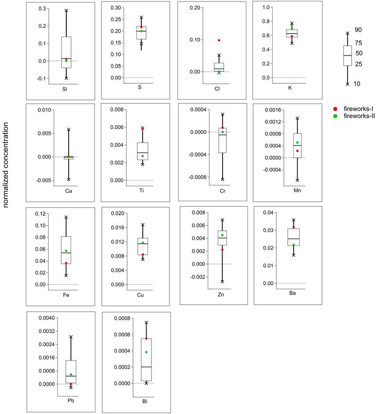
Figure S1: Unconstrained PMF with a nine-factor solution.

 2

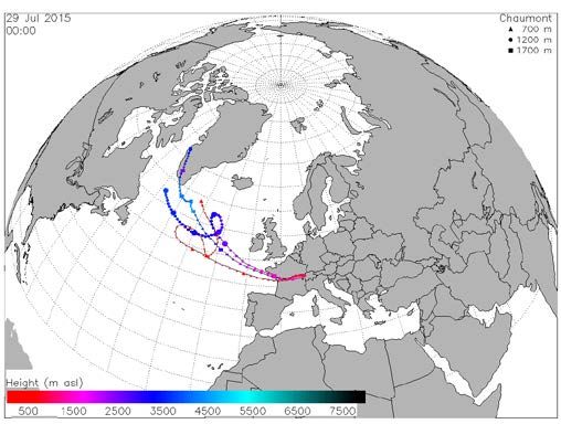
Figure S2: Box-whisker plots of Q/Q exp for the seed analysis of the nine-factor unconstrained PMF on the full dataset. Shown
 separately are the 24 solutions in which a secondary sulfate (SS) factor was identified (“SS identified”) and the 76 solutions where it
 was not (“SS not identified”).

5

 Figure S3: Histograms of the scaled residuals (e ij /s ij ) for S in the nine-factor unconstrained PMF solution on the complete dataset.

 3

Figure S4: Q/Q exp as a function of the number of factors for FH PMF analyses.

 The unexplained variation (UEV, Paatero, 2004; Canonaco et al., 2013) which is a dimensionless quantity, describes how
 5 much of the measured variation (time or variable) is not explained by each PMF factor (Eq. S1) for variable j:
 ∑ =1�� �/ �
 , = for k = 1, … … , p for � ⁄ � > 2 (S1)
 ∑ =1 ��∑ =1 | �+� ��/ �

 Where are the factor profiles and represent their time-dependent contributions. The index i represents a specific point
 in time (up to n), j is the variable, and k is a factor (up to p). are the PMF-residuals, the input data and the
 measurement uncertainties. The UEV presented here is the real UEV for high S/N threshold >2, otherwise UEV will be
10 considered as noisy UEV.

 Figure S5: Unexplained variation for each variable in FH PMF solutions: (1) constrained five-factor (black color); (2) unconstrained
 5-factor (semi filled blue color), and (3) unconstrained three-factor (blue color).

 4

This does still leave the question of how many points are too few. We test this issue with a bootstrap (BS) analysis on the FH
 dataset, which resamples the 11 data points randomly by repeating or removing data points from the original 11 data points. If
 the number of time points in the dataset were too small, one would expect a high degree of variability in the output solutions.
 5 The stability of the fireworks factor profile was assessed by investigation of 1000 random BS runs on the FH dataset (see more
 details below). Solutions were accepted based on a K / S ratio in the fireworks factor of 2.76 ± 0.5, consistent with black
 powder composition (Dutcher et al., 1999) and the concentration peak between 40 - 45 µg m-3 on 1 August 23:00 LT in the
 factor time series. This criterion yielded an acceptance rate of 21.3 %, with an average Q/Q exp of 1.3. The results of the BS
 analysis are provided in Fig. S6, where we show the fractional composition of the fireworks factor profiles from: (a) FH BS
10 analysis (blue color); (b) five-factor constrained FH PMF analysis (base case, in red color). The data and their corresponding
 uncertainty are given as box-whisker plot (bottom to top: p10-p25-p50-p75-p90) of selected 213 solutions out of 1000 BS
 runs. The displayed error bars for the base case correspond to the a-value of 0.1 used to constrain the fireworks profile in the
 complete dataset PMF analysis. This figure shows that the variation in fireworks profiles retrieved from the bootstrap analysis
 is relatively stable despite the small number of data points; indeed, it generally denotes a smaller range of values than those
15 allowed by the constrained fireworks profile in the full dataset PMF. Further, the resolved fireworks profile from FH BS
 solution agrees well with the base case, and the Q/Q exp values are reasonable. Taken together, these results suggest that the FH
 dataset contains sufficient variability to allow retrieval of a robust fireworks profile.

 Figure S6: Fireworks factor profiles from: (a) FH BS analysis (blue color); (b) five-factor constrained FH PMF analysis (base case,
20 red color). The data and their corresponding uncertainties are given as box-whisker plot (bottom to top: p10-p25-p50-p75-p90) of
 selected 213 solutions from 1000 BS runs in blue color. Base case uncertainties are given ± 10 % as error bar by considering that a-

 5

value 0.1 is applied to constrain fireworks profile in complete dataset PMF analysis. Y-axis represents the fractional composition of
 the factor profile in row-wise for each factor in ng ng-1.

 2
 
 ∑ 
 =1 ∑ =1� �
 
 Based on Q avg, defined as (n: sample time series, m: number of variables), the model explains the data variability
 ∗ 
 2
 
 ∑ 
 =1 ∑ =1� �
 
 5 very well when allowing for eight factors (Fig. S7). Furthermore, we access the change in time-dependent Q avg,i , ,
 
 when increasing the number of factors i.e., ∆Q avg,i ; contribution to Q for the (p)-factor solution minus that of the (p+1)-factor
 solution (Fig. S8). A significant decrease in ∆Q avg,i indicates that the structure in the residuals disappeared with the additional
 factor. The removed structure is evident up to eight factors. Increasing the number of factors to nine yields a new mixed factor
 of the traffic-related and background dust factors (Fig. S1). Overall, a best ME-2 solution was observed up to a number of
10 factors equal to eight.
 For the 8-factor solution, we assess how well the different variables are explained by PMF using the quantity ∆Q avg,j
 
 ∑ 
 = ∑ = � �
 
 (Fig. S9). Q avg,j shows that with 8 factors all variables are explained within their measurement uncertainty except
 
 Si and Pb. This might be linked to an underestimation of the measurement uncertainty itself.

15 Figure S7: Q avg as a function of the number of factors.

 6

Figure S8: Change in the time-dependent contribution of Q avg,i (∆Q avg,i ) as a function of the number of factors.

 7

Figure S9: Q avg as a function of variables for the eight-factor solution.

 8

Figure S10: Histograms of variables as a function of residuals weighted by the uncertainty (residual/uncertainty) for the eight-factor
 solution.

5

 9

Figure S11: a-value statistics of the accepted solutions. a-values between 0 to 0.5 were explored during BS analysis. The average a-
 value of the selected solutions was ranging from 0.2 to 0.3 for the constrained factors. The selected a-values were homogeneously
 distributed over that range.

5

 Figure S12: Time series of the sea salt and secondary sulfate factors during the fireworks period (31.07.2015-04.08.2015). The
 estimated uncertainties of the sea salt (± 42%) and the secondary sulfate (± 5%) factors during the fireworks period are added as
 error bars (standard deviation).

 10

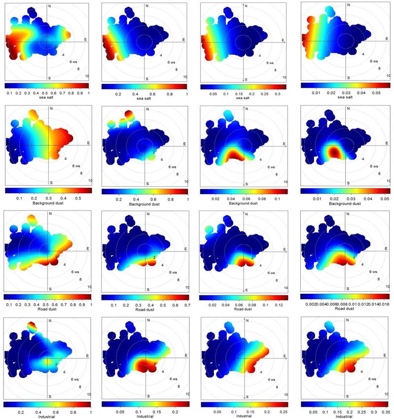
Figure S13: CBPF analysis (from left to right: 50th, 75th, 90th, 95th percentiles) of factors (sea salt, background dust, road dust,
industrial) in terms of wind speed (m s-1) and wind direction. The color code represents the probability of the factor contribution.

 11

Figure S14: Time series of the non-refractory aerosol components (measured with the ACSM), NO 2 and NO x concentration. The
 fireworks episodes are indicated in grey color.

 5 Fig. S15 provides an estimate of the overall fireworks composition and temporal variability, complementing the PMF results
 (which are shown for reference). The figure is constructed in two stages. First, the time series of fireworks contributions to
 each element is estimated by subtracting the non-fireworks factors (NFF) from the original measurements. Then, the estimated
 fireworks contribution for each element is normalized by the total fireworks element contribution, and the displayed statistics
 are calculated. This is represented mathematically below, and the expression has been added to the main text. Note that the
10 variation in fireworks profiles implied by this figure supports the representation of fireworks by 2 fireworks factors.
 x – � �
 = = (S2)
 ∑ �x – � � �
 = 

 where x represents the input data matrix for PMF, while and represent the factor time series and factor profiles driven
 by six non-fireworks factors (NFF). Here i and j denote time series and variables, respectively.

 12

Figure S15: Representation of fireworks data points (normalized concentration) in terms of median and 10-25-75-90th percentiles
 (bottom to top). Red and green dots denote the factor profiles of fireworks-I and fireworks-II, respectively.

5

 13

Figure S16: Mg / Na ratio (red bars) for 24-h filter data analysed by ICP-OES. The gray lines represent the Mg / Na ratio range
 (0.132 -0.185) in marine aerosols. The Mg / Na ratio was 0.13 and 0.16 for 28 July and 30 July, respectively while for the rest of the
 days it was higher than 0.185.

5
 Figure S17: Bottom panel: Time series of the Cl concentration from the Xact, sea salt factor (left y-axis) from the PMF solution, and
 ACSM chloride concentration (right y-axis). Top panel: Wind speed (WS in m s-1) and wind direction (WDir in degree) during the
 measurement period. The grey area in the bottom panel represents fireworks days.

 14

Figure S18: Backward trajectory (produced from the FLEXTRA Trajectory Model; https://folk.nilu.no/~andreas/flextra.html)
 analysis at different heights during a sea salt event.

5
 Figure S19: Scatter plot of Si vs. Ca scaled residuals: (a) PMF solution with one dust factor; (b) PMF solution with two dust factors.

 Figure S20: Scatter plot of Si vs. Ca.

 15

Figure S21: Mean diurnal variations of the two dust factors (left-y axis) along with wind speed and wind direction (right y-axes)
 with error bars (one standard deviation).

5

 Figure S22: Time series of the secondary sulfate factor (left y-axis) and mass concentration of SO 4 , NH 4 from the ACSM (right y-
 axis).

 16

Figure S23: Time series of equivalent concentrations of the ACSM (PM 1 ) NH 4eq , and NO 3eq and +2*SO 4eq . The NO 3eq is stacked on
 2*SO 4eq .

 References

 5 Canonaco, F., Crippa, M., Slowik, J. G., Baltensperger, U., and Prévôt, A. S. H.: SoFi, an IGOR-based interface for the efficient
 use of the generalized multilinear engine (ME-2) for the source apportionment: ME-2 application to aerosol mass spectrometer
 data, Atmos. Meas. Tech., 6, 3649–3661, https://doi.org/10.5194/amt-6-3649-2013, 2013.

 Dutcher, D. D., Perry, K. D., Cahill, T. A., and Copeland, S. A.: Effects of indoor pyrotechnic displays on the air quality in
 the Houston Astrodome, J. Air Waste Manage. Assoc., 49, 156–160, https://doi.org/10.1080/10473289.1999.10463790, 1999.

10 Paatero, P.: User’s guide for positive matrix factorization programs PMF2 and PMF3, 2004.

 17