Spatial-Channel Attention-Based Class Activation Mapping for Interpreting CNN-Based Image Classification Models

Hindawi
Security and Communication Networks
Volume 2021, Article ID 6682293, 13 pages
https://doi.org/10.1155/2021/6682293

Research Article
Spatial-Channel Attention-Based Class Activation Mapping for
Interpreting CNN-Based Image Classification Models

 Nianwen Si , Wenlin Zhang , Dan Qu , Xiangyang Luo , Heyu Chang ,
 and Tong Niu
 Information Engineering University, Zhengzhou 450001, China

 Correspondence should be addressed to Wenlin Zhang; zwlin_2004@163.com and Dan Qu; qudanqudan@163.com

 Received 4 November 2020; Accepted 1 May 2021; Published 31 May 2021

 Academic Editor: Yuewei Dai

 Copyright © 2021 Nianwen Si et al. This is an open access article distributed under the Creative Commons Attribution License,
 which permits unrestricted use, distribution, and reproduction in any medium, provided the original work is properly cited.

 Convolutional neural network (CNN) has been applied widely in various fields. However, it is always hindered by the unex-
 plainable characteristics. Users cannot know why a CNN-based model produces certain recognition results, which is a vul-
 nerability of CNN from the security perspective. To alleviate this problem, in this study, the three existing feature visualization
 methods of CNN are analyzed in detail firstly, and a unified visualization framework for interpreting the recognition results of
 CNN is presented. Here, class activation weight (CAW) is considered as the most important factor in the framework. Then, the
 different types of CAWs are further analyzed, and it is concluded that a linear correlation exists between them. Finally, on this
 basis, a spatial-channel attention-based class activation mapping (SCA-CAM) method is proposed. This method uses different
 types of CAWs as attention weights and combines spatial and channel attentions to generate class activation maps, which is
 capable of using richer features for interpreting the results of CNN. Experiments on four different networks are conducted. The
 results verify the linear correlation between different CAWs. In addition, compared with the existing methods, the proposed
 method SCA-CAM can effectively improve the visualization effect of the class activation map with higher flexibility on
 network structure.

1. Introduction reliability to gain the trust of the end-user. Research on
 interpretability of CNN has shown significant advance in
Deep-learning methods have made substantial progress in fields such as recommendation systems [12], intelligent
recent years, among which convolutional neural network medical treatment [13], and autonomous driving [14, 15].
(CNN) has been very effective for tasks like image classi- Feature visualization of a trained CNN model is a
fication [1, 2], speech recognition [3], and natural language common way to display the features learnt internally and to
processing [4]. However, owing to the end-to-end “black explain the reasons behind CNN decision-making. The most
box” nature of the CNN-based models, the knowledge direct approach is visualizing the feature maps of each layer
storage and processing mechanism of the middle layer re- [16], which can lead to visual observation of the features
mains unknown. Thus, the internal features and the basis of learnt inside CNN. Zhou et al. [8] proposed a class activation
external decision-making by CNN cannot be known clearly, mapping (CAM) method for interpreting CNN predictions,
affecting its application to some extent, especially for safety- which inserts a global average pooling (GAP) layer into
critical domains. An increasing number of studies [5–11] ordinary CNN to construct the all convolutional network. In
have been conducted recently with an aim to explore the this network, they successfully correlated CNN classification
“black box” model, focusing on the explainability of CNN’s results with the features of the middle layer by using the
decision. The purpose was to allow CNN to produce the weighted summation among the last convolutional feature
decision result while providing by itself the reason associated maps, which can be used to generate class activation map to
with the result. This would provide explainability and locate the important features contributing most to a specific

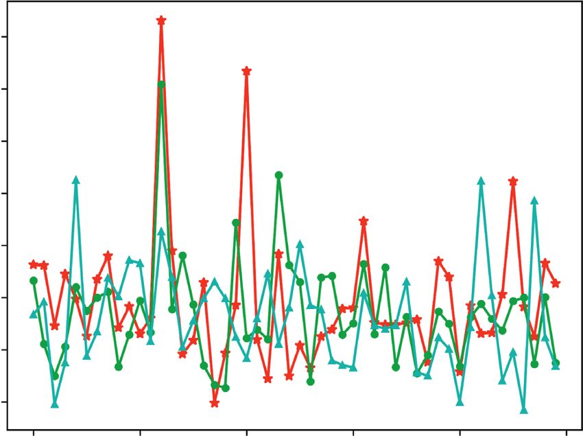
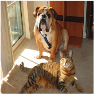
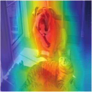
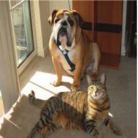
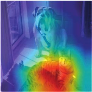
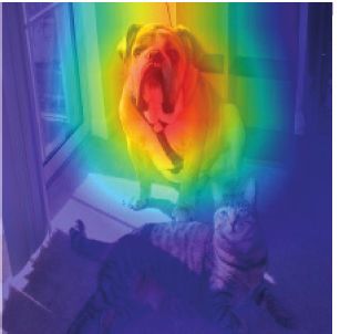
2 Security and Communication Networks

CNN prediction. Due to the utilization of GAP layer, this outputs in ResNet-18 [1] from the lower layers to the higher
method can be named GAP-CAM. The class activation map layers. The high-level feature representation is more abstract
is a class-related heatmap. The highlighted areas in the map than the lower-level one. The feature map of the highest layer
indicate the relevant regions that can activate a certain (Figure 1(f)) can locate salient features with semantic con-
output class of CNN. Selvaraju et al. [9] proposed an im- ceptual information, indicating that the feature learning of the
proved version, gradient-weighted CAM (Grad-CAM), to network is effective. Figure 1(g) shows the result of the feature
solve the limitation of GAP-CAM on network architecture. map visualization, which uses the feature map of the highest
Grad-CAM generalizes well for most CNNs and reaches a layer overlay on the original image. Feature map visualization
better localization effect on salient features. directly sums the corresponding positions of each channel of
 A detailed study on the above three feature visualization the feature map to obtain a two-dimensional image. At this
methods leads us to a new finding. We demonstrate that they time, it is equivalent to assigning a value of 1 to the weight of
are essentially the same as all of them use channel attention on each channel, which means that the importance of each
feature maps to generate class activation map. The only channel to the decision result is the same. Therefore, it is
difference among them is just the attention weight used across unable to determine the relevance of these salient features to
channels. Based on this finding, in this paper, a spatial- the current decision results. In other words, feature map
channel attention-based class activation mapping method visualization is class-independent and cannot effectively ex-
called SCA-CAM was proposed to improve the visual effect plain the results of CNN.
and produce better heatmap for interpreting CNN decisions.
The contributions of this paper can be as follows. 2.2. GAP-CAM. In order to understand the decisions made
 First, a unified feature visualization framework based on by CNN, Zhou et al. [8] made use of feature map weighted by
CAM is presented for interpreting CNN classification re- softmax weight to generate a class-specific heatmap, that is,
sults. The framework summarizes the representation of the class activation map. This heatmap can locate the dis-
three methods of feature map visualization, GAP-CAM, and criminative features of the target regions, which can support
Grad-CAM and thus has certain versatility for them. the current classification results. Shown in Figures 2(c) and
 Second, based on this visualization framework, we give 2(d) are the respective heatmaps of ResNet-18 related to
the notion of class activation weight (CAW) with respect to “dog” and “cat,” generated by GAP-CAM. The key regions
the class activation mapping for the first time. Through the are highlighted to indicate that the features of these regions
analysis of different situations, the correlation between are most relevant to the current decision.
different CAWs under multiple pooling methods is sys- To clearly describe the details of GAP-CAM, we use a
tematically deduced, and its important role in the generation basic CNN structure for comparison. Figure 3 shows the
of class activation map is determined. structure of VGGNet-16 [18] containing 13 convolutional
 Third, to take advantage of different CAWs, a new vi- layers and 3 fully connected layers, given a three-channel
sualization method called SCA-CAM is proposed. This input image with size 224 × 224 × 3, where 224 denotes the
method combines different CAWs through attention height and width. The feature map size of the last convolu-
mechanism and makes use of channel features and spatial tional layer is 7 × 7 × 512 (after maxpooling layer). Figure 4
distribution features of the feature map to generate class shows the structure of modified VGGNet-16 based on GAP-
activation map. Experimental results show that, compared CAM. Compared with the original VGGNet-16, the last
with the existing methods, it achieves better visualization maxpooling layer and the fully connected layers are removed
effects. Furthermore, it is not limited by the network from the modified network and, instead, a convolutional
structure, thereby offering higher flexibility. layer, a global average pooling (GAP) layer, and a softmax
 layer are added. The GAP layer averages the entire feature
2. Related Work map into a single value. The yellow layer in Figure 4 indicates
 the added convolutional layer with K kernels, having a kernel
The feature maps of CNN encoded by the hidden layers at size of 3 × 3, a stride of 1, and a padding of 1. In this network,
different levels have different focuses. Lower layers learn the process of generating the class activation map Hcw is
local basic features of the object, such as edges and lines, shown by the dashed line. This process denotes a weighted
while those of higher layers learn global complex features, sum between the neuron weights of a certain class in softmax
such as shapes and objects [10, 16, 17]. Therefore, the feature layer and each channel of the highest-layer feature maps.
maps can be regarded as the feature space extracted from the
input image. Visualizing the feature map is helpful in un-
derstanding the internal representation of CNN and the 2.3. Grad-CAM. Although GAP-CAM is simple, its effect is
feature maps at different layers have different applications in substantial. However, the disadvantage lies in its dependence
feature visualization. on the GAP layer, which is not always included in all CNN
 structures. Therefore, it is necessary to modify the CNN
 structure as shown in Figure 4 when using GAP-CAM,
2.1. Feature Map Visualization. Direct visualization of fea- which is a little bit complicated in application. In addition,
ture maps can help observe the representation of each middle using global pooling on feature maps will lose a lot of se-
layer of CNN. As shown in Figure 1, there are two obvious mantic information, which will degrade the performance
objects in the original image. Figures 1(b) to 1(f) display the compared to the original CNN.

Security and Communication Networks 3

 (a) (b) (c) (d)

 (e) (f ) (g)

Figure 1: ResNet-18 network: the feature maps of the middle layer ((b)∼(f ), where conv1 denotes the first convolutional layer and
conv2_x ∼ conv5_x denote the special designed convolutional modules in ResNet-18). The feature map visualization of the highest
convolutional layer (g). (a) Original image; (b) conv1; (c) conv2_x; (d) conv3_x; (e) conv4_x; (f ) conv5_x; (g) feature map visualization.

 (a) (b) (c) (d) (e) (f )

Figure 2: ResNet-18 network: the feature map visualization of the highest convolutional layer (subfigure (b)). The class activation map
visualization of GAP-CAM (c, d) and Grad-CAM (e, f ). (a) Original image; (b) feature map visualization; (c) GAP-CAM:dog; (d) GAP-
CAM:cat; (e) Grad-CAM:dog; (f ) Grad-CAM:cat.

 Feature maps of the last
 convolutional layer
 Softmax
 Input image M0

 M1
 C O N V Flatten
 …

 …

 …
 …

 M511
 224 × 224 × 3
 25088 × 1 4096 × 1 1000 × 1
 7 × 7 × 512
 Figure 3: Network structure of VGGNet-16.

 To solve the limitation of GAP-CAM in network 3. Proposed Method
structure, Selvaraju et al. [9] proposed Grad-CAM. Grad-
CAM does not need to change the network structure; in- 3.1. The Unified CNN Visualization Architecture Based on
stead, it calculates the gradient of a certain class score with CAM. The presentations of the previous section reveal that
respect to the pixel of the feature map and subsequently the three methods (feature map visualization, GAP-CAM,
averages the gradients of each channel to obtain channel- and Grad-CAM) all use heatmap to highlight the key regions
wise weight. Figures 2(d) and 2(e), respectively, denote the of the image to identify the features learnt by CNN and
heatmaps for “dog” and “cat” generated by the Grad-CAM. interpret its outputs. As shown in Figure 6, the heatmap
Figure 5 shows the process of generating the class activation generation process of them is basically the same. They all use
map using Grad-CAM on VGGNet-16. For Grad-CAM, the weighted sum between the highest-level feature map
there is no need to retrain the network and update the channels and the corresponding weights. Here, the weight
parameter, which significantly improves its efficiency. used in feature map visualization is a fixed value without

4 Security and Communication Networks

 wc1, wc2, …, wcK

 Feature maps of the last
 convolutional layer
 Softmax

 M0 GAP wc0
 Input image
 wc1 c
 M1

 C O N V

 …

 …
 …
 MK–1
 224 × 224 × 3

 14 × 14 × K K×1 1000 × 1

 Hcw = ∑wck MK
 k

 Figure 4: Modified network structure of VGGNet-16 and process of GAP-CAM.

 Backpropagation
 Feature maps of the last
 convolutional layer
 Softmax
 Input image M0

 c
 M1
 C O N V Flatten

 …

 …

 …
 …

 M511
 224 × 224 × 3
 512 × 7 × 7 25088 × 1 4096 × 1 1000 × 1

 Gc0

 Gradient matrices Gc1 GAP
 Hcg = ∑g cavg, k Mk
 of class c k
 …
 …

 Gc511
 gcavg
 7 × 7 × 512
 Figure 5: Process of Grad-CAM on VGGNet-16.

 Overlaid
 feature
 maps
 1 1 1
 wc0 • M0 + wc1 • M1 + … + wcK–1 • MK–1 = CAM

 g cavg, 0 g cavg, 1 g cavg, K – 1 Grad-
 Channel 1 Channel 2 Channel K
 CAM

 Figure 6: Unified framework of class activation map generation process.

class information, while weighs of other two methods the other two visualization methods. Direct superposition of
contain class-specific information. feature maps used in feature map visualization is equivalent
 The process shown in Figure 6 can be formulated as follows: to setting the weight of each channel to 1. The CAWs used by
 GAP-CAM and Grad-CAM are not the same, resulting in
 Hcw � wc0 · M0 + wc1 · M1 + · · · + wcK−1 · MK−1 . (1)
 different weights for each feature map channel. Therefore,
 Equation (1) represents the particular case where the different CAWs cause diverse visualization effects. From
CAW is wc � (wc0 , wc1 , . . . , wcK−1 ), c represents the class, and another perspective, feature map visualization, GAP-CAM,
K represents the number of channels. The same applies to and Grad-CAM can all be regarded as methods using a

Security and Communication Networks 5

channel attention mechanism for feature maps and where gcl,i j denotes the gradient of the pixel at (i, j) in the
assigning different attention weights to each channel. Ap- (l + 1)th channel. Thus, the averaged gradient gcavg,l of this
parently, different attention weight distributions lead to channel is obtained as follows:
different interpretation effects of class activation maps.
 1
 gcavg,l � gc . (5)
3.2. Class Activation Weight. By comparing the above three ij i,j l,i j
methods, it is observed that the CAWs, wc in GAP-CAM and
gcavg in Grad-CAM, play a key role in the generation of the Note that these gradients come from the derivatives of a
class activation map and determine the effect of visualization specific class score, containing features associated with the
to some extent. Therefore, to analyze the function of CAWs class. At this point, the average gradient
used in GAP-CAM and Grad-CAM in detail, in this section, gcavg � (gcavg,0 , gcavg,1 , . . . , gcavg,K−1 ). Each channel is just the
we first study the relationship between the two kinds of CAW used in Grad-CAM.
CAWs in CNN structure with a GAP layer and subsequently From equations (2)–(5), the relationship between the
remove the GAP layer for further analysis. two kinds of CAWs, wc and gcavg , is given by
 1 c
3.2.1. CNN CAW with a GAP Layer. GAP layer is commonly gcavg,l � w. (6)
 ij l
used in modern CNNs [1, 19, 20] which often appears before
the fully connected layer. It is also the core component of From equation (6), in a CNN with a GAP layer, there
GAP-CAM. We choose the CNN with a GAP layer. In this exists a linear relationship between the two kinds of CAWs.
way, GAP-CAM and Grad-CAM can be unified into one Intuitively, as illustrated in Figure 7, the forward process
network without modifying the network structure. In a CNN from the multichannel feature map to the score vector only
with a GAP layer, the feature extraction and classification includes a GAP operation, which is a linear calculation.
process over the input image is illustrated in Figure 7. Thus, the relationship between the two kinds of CAWs is
 Given an input image, the last convolutional feature map linear. The class activation maps in Figures 2(c) and 2(e) and
M � (M0 , M1 , . . . , MK−1 ) is obtained after feature extrac- Figures 2(d) and 2(f ) are quite similar, which also verifies
tion. Afterwards, it is fed into the GAP layer to obtain the this linear correspondence.
feature vector (m0 , m1 , . . . , mK−1 ). Finally, the score vector
(y0 , y1 , . . .) of all classes in the classification layer (before
softmax) is obtained. This process can be formulated as 3.2.2. CNN CAW without the GAP Layer. GAP layer just
 c
Ml ⟶ GAP ml ⟶wl yc , where Ml denotes the l + 1(l � 0, 1 employs a special kind of pooling strategy, in which the
, . . . , K − 1) channel of M, ml is the pooled value of Ml , and window size corresponds to the feature map size. For other
yc denotes the score of class c, which can be computed as pooling methods in self-designed CNN, such as average
follows: pooling and maxpooling, a smaller window size (e.g., 2 × 2 or
 3 × 3) is usually selected to reduce the dimension of the
 yc � wcl ml , (2) feature map and also retain more semantic information. In
 l
 this case, the relationship between the two kinds of CAWs is
where wcl represents the weight connecting ml and the more complex and should be analyzed for different
neuron of class c in the classification layer. According to the situations.
GAP process, ml can be computed as follows: To facilitate analysis, a 4 × 4 × 3 sized feature map is used
 as an example. The detailed process is illustrated in Figure 8.
 1
 ml � GAP Ml � M , (3) The 4 × 4 × 3 sized feature map is pooled using four different
 ij i,j l,i j pooling methods to output feature vectors. Afterwards, the
 feature vectors are fed into the classification layer to obtain
where Ml,i j denotes the pixel at the spatial location (i, j) in the binary classification scores, y0 and y1 (before softmax).
the (l + 1)th channel and GAP() represents the global av- In this process, the four following different pooling methods
erage pooling on the feature map Ml . From equations (2) are, respectively, used:where the CAW, g1avg , is still a linear
and (3), the score yc depends on both the pixel value Ml,i j of combination of the elements of w1 . Here, the number of
the feature map and the weight wc of the classification layer. summed elements and the coefficient are still the same as
At this point, the weight wc � (wc0 , wc1 , . . . , wcK−1 ) is just the those of case B.
CAW used in GAP-CAM.
 Moreover, the CAW used in Grad-CAM can be obtained A GAP. The window size of pooling corresponds to the
using the gradient-based backpropagation process. To feature map size. According to the analysis in the
achieve this, the score yc is backpropagated into the feature previous subsection, the relationship between CAWs is
space of the last convolutional layer to compute its gradients as follows:
with respect to the pixels in the feature map:
 zyc 1 c
 gcl,i j � , (4) gcavg,l � w, c � 1, 2; l � 1, 2, 3, (7)
 zMl,i j 4×4 l

6 Security and Communication Networks

 Fully
 Convolution GAP connected
 Multichannel
 Input image Feature vector Output class
 feature map
 Feature Pooling Classification
 extraction
 (M0, M1, ..., MK–1) (m0, m1, ..., mK–1) (y0, y1, ...)
 Figure 7: Classification process of the CNN with a GAP layer.

 GAP Flatten m0 w10 y0
 Therefore, the gradients of y1 with respect to the feature
 m1 w11
 m2 y1 map pixels are related to the weights of the classification
 (4, 4) 1×1×3 w12
 3×1 layer. Using equations (4) and (5), the average gradients
 M2 Avgpool Flatten m0 w10 of each feature map channel are computed:
 m1 w1 y0
 M1 1 y1
 (2, 2)/2

 …
 M0 2×2×3 1
 12 × 1
 g1avg,0 � w1 , s � 0, 1, 2, 3, (13)
 Maxpool Flatten m0 w10 y0 4×4 s s
 m1 w11 y1
 4×4×3 (2, 2)/2
 …

 2×2×3
 12 × 1 1
 g1avg,1 � w1 , s � 4, 5, 6, 7, (14)
 Avgpool Flatten m0 w10
 y0 4×4 s s
 m1
 w11 y1
 (2, 2)/1
 …

 1
 3×3×3 27 × 1
 g1avg,2 � w1 , s � 8, 9, 10, 11. (15)
 4×4 s s
 Figure 8: Process of four different pooling methods.

 In this case, the CAW, g1avg � (g1avg,0 , g1avg,1 , g1avg,2 ), is a
 where there is a linear relationship between the two linear combination of the elements of the weight
 CAWs, whose coefficient is the reciprocal of the feature w1 � (w10 , w11 , . . . , w115 ). The number of elements
 map size. summed is the same as the number of elements in each
 B Average pooling (2, 2)/2. The window size is set to (2, feature map channel obtained from pooling and the
 2) and stride 2. Then, the score y1 can be computed as coefficient value of the linear combination is still the
 follows: reciprocal of the size of the feature map.
 CMaxpooling (2, 2)/2. The window size is set to (2, 2)
 and stride 2. In this case, we get the same conclusion as
 y1 � w1s ms , s � 0, 1, . . . , 11, (8) that in case B.
 s
 ➃ Average pooling (2, 2)/1. The window size is set to (2,
 2) and stride 1. In this case, although there exists
 where m0 ∼ m3 , m4 ∼ m7 , and m8 ∼ m11 can be ob- gradient superposition at the positions of stride over-
 tained using M1 , M2 , and M3 , respectively. According lap, we can compute the average gradients through each
 to the average pooling process, we can compute the channel of the feature map:
 value of m0 ∼ m3 as follows:
 1
 g1avg,0 � w1 , s � 0, 1, . . . , 8, (16)
 1 4×4 s s
 m0 � M , i � 0, 1; j � 0, 1, (9)
 2 × 2 i,j 0,i j
 1
 g1avg,1 � w1 , s � 9, 10, . . . , 17, (17)
 4×4 s s
 1
 m1 � M , i � 0, 1; j � 2, 3, (10)
 2 × 2 i,j 0,i j 1
 g1avg,2 � w1 , s � 18, 19, . . . , 26, (18)
 4×4 s s
 1
 m2 � M , i � 2, 3; j � 0, 1, (11)
 2 × 2 i,j 0,i j Although the GAP layer in CNN was not used, the above
 results show that there still exists a linear relationship be-
 1 tween the two CAWs. In this linear relationship, the CAW,
 m3 � M , i � 2, 3; j � 2, 3. (12) g1avg , is always the linear combination of the elements of the
 2 × 2 i,j 0,i j
 CAW w1 , and the coefficient value of the linear combination
 is always the reciprocal of the feature map size. In other
 Similarly, m4 ∼ m11 can be computed using the above words, the two kinds of CNN CAWs are always consistent.
 process. From equations (8)–(12), we know that y1 is Therefore, it is natural to combine them together to fine-tune
 obtained using the weight w1s of the classification layer the generation process of a class activation map for better
 and the pixel values Ml,i j of the feature maps. visualization effect.

Security and Communication Networks 7

3.3. Spatial-Channel Attention-Based CAM. In the above this channel. The order of the two attention weights does not
analysis, we know that the role of a CAW is equivalent to that affect the final result.
of a channel-wise attention weight. It performs adjustment In the CNN with a GAP layer, there is a linear rela-
across channels to synthesize a class activation map. Con- tionship between the two CAWs, wc and gcavg . Therefore,
sidering the consistency of the two CAWs, we propose combining equation (5) and (6), equation (21) can be
spatial-channel attention-based class activation mapping simplified as
method called SCA-CAM. By combining the spatial and
 Hcsc � gc0,i j gc0 · M0 + gc1,i j gc1 · M1 + · · · + gcK−1,i j gcK−1 · MK−1 .
channel attentions, the positions and channels with high i,j i,j i,j
relevance to the current classification are strengthened,
 (22)
while those with low relevance are further suppressed. The
process is shown in Figure 9. In equation (22), both the spatial attention and channel
 attention weights are composed of gradients.
 In the CNN without the GAP layer, when avgpool (2, 2)/
3.3.1. Spatial Attention. For a single channel of the highest- 2 or maxpool (2, 2)/2 is adopted for pooling, the attention
level feature map, the spatial distribution of semantic fea- weight of the first channel can be obtained from equations
tures varies enormously across pixel positions. These spatial (5) and (13):
distribution features of pixels cannot be well utilized by
 1 1
using channel attention alone as in GAP-CAM and Grad- gcavg 0 � gc � wc , s � 0, 1, 2, 3; c � 1,
CAM. Therefore, the spatial attention mechanism is adopted ij i,j 0,i j
 ij s s
in this study to realize different weights at different positions (23)
of each channel to take advantage of this spatial distribution
feature. Specifically, by calculating the gradient of each pixel where s represents the element number in the pooled feature
in the feature map, a class-specific spatial attention weight map. In this case, ignoring the influence of the coefficient
matrix, namely, a pixel-level gradient matrix, can be ob- 1/ij, the channel attention weight s w1s can still be replaced
tained as follows: by the pixel-level gradients:
 gc � gc0 , gc1 , . . . , gcK−1 ∈ RK×H×W , (19) wcs � gc0,i j , s � 0, 1, 2, 3; c � 1. (24)
 s i,j
 gcl
where ∈ R H×W
 denotes the (l + 1)th channel of the gra-
dient matrix and each element is a pixel’s gradient with Therefore, in this case, equation (22) is still right.
respect to the score of class c. This matrix contains both the Similarly, when using the methods of avgpool (2, 2)/1,
important features of each spatial position and the features equation (22) can still be derived from equations (5) and
related to the output class, which can achieve a pixel-level (16).
attention weight. In conclusion, under the unified framework presented in
 Figure 6, SCA-CAM can be formulized using equation (22).
 It combines the advantages of spatial and channel attention
3.3.2. Channel Attention. In channel attention mechanism, weight and integrates the representation of the two CAWs,
each channel is regarded as a whole. Each channel corre- under different pooling methods, into a unified form. As a
sponds to a different feature and contributes differently to consequence, there is no need to rely on softmax weight,
different output classes. Therefore, different attention which simplifies the process while making use of more
weights should be assigned to each channel when generating features.
the class activation map. Note that, in literatures [6, 21] and [22], channel at-
 tention or spatial-channel attention mechanism was added
 wc � wc0 , wc1 , . . . wcK−1 ∈ RK , (20) in CNN. The attention weight was adjusted along with the
 network parameters to improve the performance of CNN
where wcl ∈ R represents the channel attention weight of the
 classification. In contrast, the proposed SCA-CAM only
(l + 1)th channel related to class c.
 realizes visual interpretation of CNN output. The attention
 weight used in this study is composed of gradients and can
3.3.3. Combining Spatial and Channel Attention. be obtained offline without network training. This is also a
According to the unified framework presented in Section 3.1, difference between SCA-CAM and other methods.
the spatial attention weights gc and the channel attention
weights wc are combined to generate the class activation map 4. Results and Analysis
as follows:
 The pretrained image classification models used in the ex-
 Hcsc � wc0 gc0 · M0 + wc1 gc1 · M1 + · · · + wcK−1 gcK−1 · MK−1 , periments are provided by torchvision package [23, 24],
 (21) including SqueezeNet [25], ResNet-18 [1], ResNet-50 [1],
 and DenseNet-161 [19]. These networks were trained to the
where Ml ∈ RH×W denotes the (l + 1)th channel of the best performance on the ImageNet dataset [26]. The error
feature map; gcl represents the spatial attention weight matrix rates of them are listed in Table 1. Theoretically, models with
of this channel; wcl represents the channel attention weight of better performance show stronger ability for feature

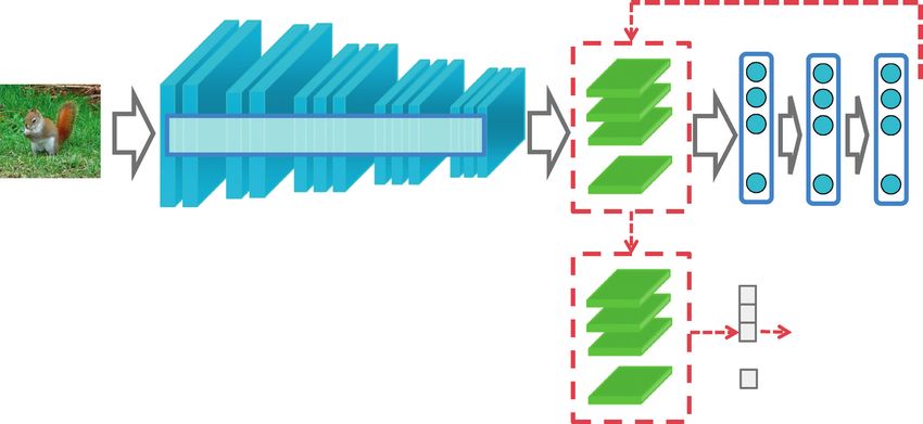
8 Security and Communication Networks

 CAW gc CAW wc

 ts
 ien Spatial attention
 ad
 Gr Channel attention

 .

 Feature map Activation map
 Figure 9: Process of SCA-CAM.

Table 1: Error rates (%) [23] of four different networks on Table 2: The top five classification results of the four networks.
ImageNet dataset and feature map size of the last convolutional
layer. No. C P
 SqueezeNet
Network Top-1 error Top-5 error Feature map size 1 Tiger cat 0.378
SqueezeNet 41.81 19.38 13 × 13 × 1000 2 Bullmastiff 0.350
ResNet-18 30.24 10.92 7 × 7 × 512 3 Great Dane 0.102
ResNet-50 23.85 7.13 7 × 7 × 2048 4 Boxer 0.071
DenseNet-161 22.35 6.20 7 × 7 × 2208 5 Tabby 0.023
 ResNet-18
 1 Boxer 0.426
representation and location of key features. Because the
 2 Bullmastiff 0.265
feature visualization aims to interpret the pretrained CNN 3 Tiger cat 0.175
classification results, network training is not required. 4 Tiger 0.094
 5 American Staffordshire Terrier 0.014
4.1. Visualization and Comparison of the CAWs. CAW is ResNet-50
important for generating the heatmap. As mentioned above, 1 Bullmastiff 0.384
 2 Tiger cat 0.168
the CAWs can be divided into two types: in GAP-CAM,
 3 Boxer 0.094
CAW denotes the weight of softmax layer, and in Grad- 4 Tabby 0.059
CAM, CAW denotes the averaged gradient of each channel 5 Doormat 0.050
for a particular class score. To obtain the CAW, given the DenseNet-161
input image shown in Figure 1, the predictions are shown in 1 Bullmastiff 0.679
Table 2, where C denotes the class name and P denotes the 2 Boxer 0.227
corresponding probability. 3 Doormat 0.035
 4 Tiger cat 0.015
 5 French bulldog 0.010
4.1.1. Comparison of the Different CAWs for the Same Output
Class. The two types of CAWs of each network are illus-
trated in Figure 10. Taking the SqueezeNet as an example, horizontal axis represents each feature map channel (ran-
the weights corresponding to 50 channels were randomly domly selected) and the vertical axis represents the size of the
selected from the 1000 channels. Because the gradient value two kinds of CAWs, corresponding to the channel. Obviously,
is infinitesimal and has a large difference from the weight there is a correspondence between the two CAWs and, in
value of the classification layer, the average gradient value addition, the numerical values always show the same fluc-
increased by 100 times during the mapping to facilitate the tuation, indicating that a linear relation exists. Similarly,
comparison, which will not affect the comparison. There are Figures 10(c)–10(h) represent the corresponding CAWs of
two types of CAW shown in Figure 10: other three networks. Again, a similar linear relation is ob-
 (1) Softmax weight: It represents the weight of a certain served. More precisely, to calculate the correlation coefficient
 neuron (class) in the softmax classification layer, that between each pair of curves, the softmax weight is divided by
 is, the first CAW. the average gradient to obtain the specific values of the
 correlation coefficient: αSqueezeNet � 1 · 72, αResNet−18 � 0 · 49,
 (2) Average gradient: It indicates the gradient average of the
 and αResNet−50 � 0 · 49. Because the DenseNet-161 adds a
 feature map for a certain class, that is, the second CAW.
 ReLU layer after the last convolutional feature map, the
 Figures 10(a) and 10(b), respectively, show the corre- gradient of the backpropagation also passes through this layer,
sponding two types of CAWs with respect to “tiger cat” and so the result is slightly different from the other three networks
“bull mastiff,” classified by SqueezeNet. Among them, the and does not reflect a strictly consistent correlation.

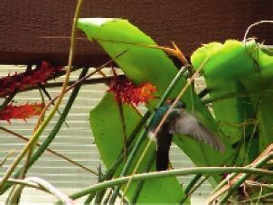
Security and Communication Networks 9

 SqueezeNet SqueezeNet ResNet-18 ResNet-18
 0.100 0.5 0.2
 0.10 0.4
 0.075
 0.1
 0.050 0.3
 0.05
 0.2
CAW

 CAW

 CAW

 CAW
 0.025
 0.0
 0.00 0.000 0.1

 –0.025 0.0 –0.1
 –0.05
 –0.050 –0.1
 –0.2
 –0.075 –0.2
 –0.10
 0 10 20 30 40 50 0 10 20 30 40 50 0 10 20 30 40 50 0 10 20 30 40 50
 Channel Channel Channel Channel

 Softmax weight Softmax weight Softmax weight Softmax weight
 Average gradient Average gradient Average gradient Average gradient

 (a) (b) (c) (d)
 ResNet-50 ResNet-50 DenseNet-161 DenseNet-161
 0.25 0.20 0.10 0.125

 0.20 0.100
 0.15
 0.05
 0.15
 0.075
 0.10
 0.10
 0.00 0.050
CAW

 CAW

 CAW

 CAW
 0.05 0.05
 0.025
 0.00 0.00 –0.05
 0.000
 –0.05
 –0.05 –0.10 –0.025
 –0.10
 –0.10 –0.050
 0 10 20 30 40 50 0 10 20 30 40 50 0 10 20 30 40 50 0 10 20 30 40 50
 Channel Channel Channel Channel

 Softmax weight Softmax weight Softmax weight Softmax weight
 Average gradient Average gradient Average gradient Average gradient

 (e) (f ) (g) (h)

Figure 10: Visualizations of CAWs in SqueezeNet, ResNet-18, ResNet-50, and DenseNet-161. (a) CAW of “tiger cat,” (b) CAW of
“bullmastiff,” (c) CAW of “boxer,” (d) CAW of “tiger cat,” (e) CAW of “bullmastiff,” (f ) CAW of “tiger cat,” (g) CAW of “bullmastiff,” and
(h) CAW of “tiger cat.”

4.1.2. Comparison of the Same CAWs for Different Output From a horizontal perspective under the same CNN, the
Classes. Considering the two CAWs separately, the channel localization effect of the proposed SCA-CAM is better than
weight values for different output classes are shown in Fig- that of GAP-CAM and Grad-CAM. Because the attention
ure 11. For ResNet-18 network, the predictions of the top three weight of SCA-CAM contains two types of CAWs, this
classes are, respectively, boxer � 0.426; bull mastiff � 0.265; and method offers better performance in distinguishing regions
tiger cat � 0.175. Figure 11(a) shows the visualization of the of interest.
softmax weight corresponding to the top three classes. Simi- From a vertical perspective, under the same feature
larly, Figure 11(b) illustrates the average gradients corre- visualization method, the localization effects under
sponding to the top three classes. In Figure 11, for the CAW of different networks are shown for comparisons. In Ta-
the same type, the corresponding weight values of different ble 1, the error rates of the four networks are in the
output classes vary considerably on the same channel, indi- following order: SqueezeNet > ResNet-18 > ResNet-
cating that the contribution of the channel to each output class 50 > DenseNet-161. The results shown in Figure 12 in-
is significantly different. Owing to the difference in the weight, dicate that the higher the accuracy of the network, the
the weighted summation between the weight and the feature better the localization effects of the heatmap. Intuitively,
map can produce different class activation region effects. the improved CNN makes the feature maps more focused
Concurrently, a horizontal comparison of the weight curves on the target object and leads the network to learn more
corresponding to each class in Figures 11(a) and 11(b) further comprehensive features. Therefore, the heatmap gener-
verifies the conclusions of the previous section. ated on CNN with a high accuracy is better than those
 with a low accuracy.

4.2. Visual Effects of the Different Methods. Here, we will
inspect the localization effect of the class activation map 4.3. Class Discriminative Visualization Using SCA-CAM.
generated by SCA-CAM and make comparisons with those The CAWs used by SCA-CAM are directly related to the
of other methods. For the same input image, the visuali- output classes. Therefore, SCA-CAM can visualize the fea-
zation effects of three methods, GAP-CAM, Grad-CAM, and tures of a specific class and locate the region of interest
SCA-CAM, are compared under four CNNs: SqueezeNet, related to the class. Figure 13 shows the visual interpretation
ResNet-18, ResNet-50, and DenseNet-161. All of these four of DenseNet-161 output class. For image 1, the top five
CNNs contain a GAP layer (or a layer with the same function classes are as follows: flowerpot � 0.270; little blue
as GAP layer) in their structure. Therefore, according to the heron � 0.148; hummingbird � 0.069; walking stick � 0.062;
analysis in Section 3.2, GAP-CAM and Grad-CAM can be and bulb � 0.051. For image 2, the top five classes are as
used simultaneously for comparison. Results are shown in follows: studio couch � 0.860; bookcase � 0.118;
Figure 12. library � 0.010; rocking chair � 0.003; and table lamp � 0.002.

10 Security and Communication Networks

 0.25 0.5
 0.20 0.4

 CAW (average gradient)
 CAW (softmax weight)

 0.15 0.3

 0.10 0.2

 0.05 0.1

 0.00 0.0

 –0.05 –0.1

 –0.10 –0.2

 0 10 20 30 40 50 0 10 20 30 40 50
 Channel Channel
 Softmax weight 1 Average gradient 1
 Softmax weight 2 Average gradient 2
 Softmax weight 3 Average gradient 3
 (a) (b)

Figure 11: Visualizations of CAWs of ResNet-18. (a) ResNet-18: softmax weight (CAW) of the top three classes. (b) ResNet-18: average
gradient (CAW) of the top three classes.

Figure 12: Class activation maps generated by SCA-CAM, GAP-CAM, and Grad-CAM under four networks. Networks from the first row to
the fourth row are SqueezeNet, ResNet-18, ResNet-50, and DenseNet-161, respectively.

In class activation map, the most relevant image region to 4.4. Ability of Localizing the Same Object Class. Here, we
the specific class is highlighted. According to the results select multiple images of the same class and visualize the key
shown in Figure 13, the visualization effect is closely related features among them to test the ability of SCA-CAM to
to the output class, and the CAWs corresponding to various locate similar objects from the different images. Test images
classes are significantly different. Therefore, the generated come from ILSVRC 2012 dataset [26] and Tiny ImageNet
maps can realize the interpretation of specific output classes. [27]. Images selected from Tiny ImageNet dataset can be
Also, the visualization effect is independent of the score used to test the transferability of the proposed method.
corresponding to this class. This means that the probability Shown in Figure 14 are the results on different images
that an image belongs to this class will not influence its visual belonging to four classes, each of “airliner,” “hartebeest,”
interpretation. “spider,” and “butterfly.” The results indicate that, for the

Security and Communication Networks 11

 Image 1 Flowerpot Little blue heron Hummingbird Walking stick Bulbul

 Image 2 Studio couch Bookcase Library Rocking chair Table lamp
 Figure 13: Visualizations of class activation maps for different classes.

 (a) (b)

 (c) (d)

Figure 14: Visualizations of the same object class in different images. Images in the first row are from ILSVRC 2012 dataset, and images in
the second row are from Tiny ImageNet dataset. (a) Airliner, (b) hartebeest, (c) spider, and (d) butterfly.

images in the same class, the SCA-CAM can effectively different CAWs is found. Furthermore, a spatial-channel
locate the regions related to the target with the same class. attention-based class activation mapping method SCA-
Even for the image with multiple objects, the regions cor- CAM is proposed. Considering both channel and spatial
responding to these objects can be located simultaneously. distribution features, the proposed method combines dif-
Furthermore, for targets with very similar contexts in some ferent CAWs as attention weights, which can improve the
images, the proposed method can still find reasonable re- visual effect of the class activation map. Compared with
gions to explain the current classification results, indicating existing methods, the proposed method can effectively
that the SCA-CAM has promising robustness for images improve the effects of class activation maps and be applied to
with complex contexts. multiple CNN networks.
 The interpretability of CNN is significant for some special
5. Conclusions fields, such as smart medical care, financial lending, and au-
 tonomous driving. Only an interpretable and transparent
In this paper, a unified CNN feature visualization framework CNN-based model can support their safe use. In the future, we
based on CAM is presented. Under this framework, a de- will explore to achieve fine-grained interpretability with the
tailed analysis of the CAWs in different pooling situations is improvement of this method to reduce visual noise in heat-
conducted, and a consistent linear relationship between maps and further study the applications of it in other fields.

12 Security and Communication Networks

Data Availability [11] K. Simonyan, A. Vedaldi, and A. Zisserman, “Deep inside
 convolutional networks: visualising image classification
The datasets used in the experiment are ImageNet dataset models and saliency maps,” in Proceedings of the ICLR 2013 :
and Tiny ImageNet dataset. They can be downloaded at International Conference on Learning Representations,
http://image-net.org/download.php and http://cs231n. Scottsdale, AZ, USA, 2013.
stanford.edu/tiny-imagenet-200.zip. [12] Y. Tan, M. Zhang, Y. Liu, and S. Ma, “Rating-boosted latent
 topics: understanding users and items with ratings and re-
 views,” in Proceedings of the 25th International Joint Con-
Conflicts of Interest ference on Artificial Intelligence, pp. 2640–2646, New York,
 NY, USA, 2016.
The authors declare that there are no conflicts of interest [13] Z. Zhang, Y. Xie, F. Xing, M. McGough, and L. Yang,
regarding the publication of this paper. “MDNet: a semantically and visually interpretable medical
 image diagnosis network,” in Proceedings of the 2017 IEEE
Acknowledgments Conference on Computer Vision and Pattern Recognition,
 pp. 3549–3557, Honolulu, HW, USA, 2017.
This work was supported by the National Natural Science [14] J. Kim and J. Canny, “Interpretable learning for self-driving
Foundation of China (no. 61673395). cars by visualizing causal attention,” in Proceedings of the 2017
 IEEE International Conference on Computer Vision,
 pp. 2961–2969, Venice, Italy, 2017.
References [15] J. Chen, S. E. Li, and M. Tomizuka, “Interpretable end-to-end
 [1] K. He, X. Zhang, S. Ren, and J. Sun, “Deep residual learning urban autonomous driving with latent deep reinforcement
 for image recognition,” in Proceedings of the IEEE Conference learning,” in Proceedings of the IEEE Transactions on Intel-
 on Computer Vision and Pattern Recognition, Las Vegas, NV, ligent Transportation Systems, pp. 1–11, Blacksburg, VA, USA,
 USA, 2016. 2020.
 [2] H. Jie, S. Li, and S. Gang, “Squeeze-and-excitation networks,” [16] A. Krizhevsky, I. Sutskever, and G. Hinton, “Imagenet clas-
 in Proceedings of the IEEE Conference on Computer Vision and sification with deep convolutional neural networks,” in
 Pattern Recognition, Honolulu, HI, USA, 2017. Proceedings of the 26th Annual Conference on Neural Infor-
 [3] S. Toshniwal, T. N. Sainath, R. J. Weiss et al., “Multilingual mation Processing Systems, pp. 1106–1114, Lake Tahoe, NV,
 speech recognition with a single end-to-end model,” in USA, 2012.
 Proceedings of the IEEE International Conference on Acoustics, [17] Z. Qin, F. Yu, C. Liu, and X. Chen, “How convolutional neural
 Speech and Signal Processing, Calgary, Canada, 2018. networks see the world—a survey of convolutional neural
 [4] J. Devlin, M. W. Chang, K. Lee, and K. Toutanova, “Bert: pre- network visualization methods,” Mathematical Foundations
 training of deep bidirectional transformers for language of Computing, vol. 1, no. 2, pp. 149–180, 2018.
 understanding,” in Proceedings of the 2019 Conference of the [18] K. Simonyan and A. Zisserman, “Very deep convolutional
 North American Chapter of the Association for Computational networks for large-scale image recognition,” in Proceedings of
 Linguistics: Human Language Technologies, vol. 1, pp. 4171– the ICLR 2015: International Conference on Learning
 4186, Minneapolis, MN, USA, 2019. Representations, San Diego, CA, USA, 2015.
 [5] M. D. Zeiler and R. Fergus, “Visualizing and understanding [19] G. Huang, Z. Liu, L. V. D. Maaten, and K Q. Weinberger,
 convolutional networks, computer vision—ECCV 2014,” in “Densely connected convolutional networks,” in Proceedings
 Proceedings of the 13th European Conference on Computer of the IEEE Conference on Computer Vision and Pattern
 Vision, pp. 818–833, Zurich, Switzerland, 2014. Recognition, pp. 2261–2269, Honolulu, HI, USA, 2017.
 [6] M. T. Ribeiro, S. Singh, and C. Guestrin, “Why should I trust [20] C. Szegedy, V. Vanhoucke, S. Ioffe, J. Shlens, and Z. Wojna,
 you?: explaining the predictions of any classifier,” in Pro- “Rethinking the inception architecture for computer vision,”
 ceedings of the 2016 Conference of the North American Chapter in Proceedings of the IEEE Conference on Computer Vision and
 of the Association for Computational Linguistics: Demon- Pattern Recognition, pp. 2818–2826, Las Vegas, NV, USA,
 strations, pp. 97–101, San Diego, CA, USA, 2016. 2016.
 [7] Q. Zhang, Y. N. Wu, and S.-C. Zhu, “Interpretable con- [21] S. Woo, J. Park, J.-Y. Lee, and I. S. Kweon, “CBAM: con-
 volutional neural networks,” in Proceedings of the IEEE/CVF volutional block attention module, computer vision—ECCV
 Conference on Computer Vision and Pattern Recognition, 2018,” in Proceedings of the European Conference on Computer
 pp. 8827–8836, Salt Lake City, UT, USA, 2018. Vision, pp. 3–19, Munich, Germany, 2018.
 [8] B. Zhou, A. Khosla, A. Lapedriza, A. Oliva, and A. Torralba, [22] L. Chen, H. Zhang, J. Xiao et al., “Spatial and channel-wise
 “Learning deep features for discriminative localization,” in attention in convolutional networks for image captioning,” in
 Proceedings of the 2016 IEEE Conference on Computer Vision Proceedings of the IEEE Conference on Computer Vision and
 and Pattern Recognition, pp. 2921–2929, Las Vegas, NV, USA, Pattern Recognition, pp. 6298–6306, San Juan, PR, USA, 2017.
 2016. [23] A. Paszke, S. Gross, S. Chintala et al., “Automatic differen-
 [9] R. R. Selvaraju, M. Cogswell, A. Das, R. Vedantam, D. Parikh, tiation in pytorch,” in Proceedings of the 31st International
 and D. Batra, “Grad-CAM: visual explanations from deep Conference on Neural Information Processing Systems
 networks via gradient-based localization,” in Proceedings of (Workshop), Long Beach, CA, USA, 2017.
 the IEEE International Conference On Computer Vision,, [24] S. Marcel and Y. Rodriguez, “Torchvision the machine-vision
 pp. 618–626, Venice, Italy, 2017. package of torch,” in Proceedings of the 18th ACM Interna-
[10] B. Zhou, A. Khosla, A. Lapedriza, A. Oliva, and A. Torralba, tional Conference on Multimedia, pp. 1485–1488, New York,
 “Object detectors emerge in deep scene CNNS,” in Pro- NY, USA, 2010.
 ceedings of the ICLR 2015: International Conference on [25] F. N. Iandola, S. Han, M. W. Moskewicz, K. Ashraf, W J. Dally,
 Learning Representations, San Diego, CA, USA, 2015. and K. Keutzer, “Squeezenet: alexnet-level accuracy with 50x

Security and Communication Networks 13

 fewer parameters and