Kinematic and dinamic study of the suspension system of an electric single seater competition Formula Student - Ingenius
←
→
Page content transcription
If your browser does not render page correctly, please read the page content below
Scientific Paper / Artículo Científico
                                                                                    https://doi.org/10.17163/ings.n20.2018.09
                                                                                     pISSN: 1390-650X / eISSN: 1390-860X

        Kinematic and dinamic study of the
      suspension system of an electric single
       seater competition Formula Student
          Estudio cinemático y dinámico del
       sistema de suspensión de un monoplaza
         de competencia eléctrico Formula
                      Student
                       Christian Arévalo1,∗ , Ayrton Medina1 , Juan Valladolid1

 Abstract                                                     Resumen
 The level of competitiveness generated by Formula El nivel de competitividad que genera la Formula
 Student has led to a series of studies and technolog- Student ha desencadenado en una serie de estudios
 ical advances in order to improve the performance y avances tecnológicos con el fin de mejorar cada
 of single-seaters, so that their operation is success- vez más el rendimiento de los monoplazas para que
 ful according to the requirements of the competition. se desenvuelvan con éxito ante las exigencias de la
 This document details the study of the suspension competencia. En este documento se detalla el estu-
 system of an electric Formula Student single-seater. dio del sistema de suspensión de un monoplaza de
 This study involves an analysis of the kinematics and competencia eléctrico Formula Student. Este estudio
 dynamics of the suspension system in which an analyt- involucra un análisis de la cinemática y dinámica
 ical determination of movement, loads and vibrations del sistema de suspensión en el cual se realiza una
 is carried out by means of simulation software and determinación analítica del movimiento, cargas y vi-
 mathematical calculations. The aim of the study is to braciones por medio de software de simulación y de
 evaluate the performance of the suspension according cálculos matemáticos. Con el estudio se busca eva-
 to the regulations of the competition, to establish luar el rendimiento de la suspensión en función del
 parameters that improve the suspension system and reglamento de la competencia, con el fin de establecer
 at the same time the performance of the car in terms parámetros que mejoren el sistema de suspensión y
 of comfort and safety.                                 a la vez el desempeño del monoplaza en términos de
                                                        confort y seguridad.
 Keywords: Single seater, Suspension, Dynamics,               Palabras clave: monoplaza, suspensión, dinámica,
 Kinematics.                                                  cinemática.

1,∗
  Transport Engineering Research Group (GIIT), Automotive Mechanical Engineering Major, Universidad
  Politécnica Salesiana, Cuenca – Ecuador. Author for correspondence ): carevalom@est.ups.edu.ec.
    https://orcid.org/0000-0002-2906-3553,    https://orcid.org/0000-0002-9172-7568,
    https://orcid.org/0000-0002-3506-2522.
Received: 13-04-2018, accepted after review: 19-06-2018
Suggested citation: Arévalo, C.; Medina, A. and Valladolid, J. (2018). «Kinematic and dinamic study of the suspension
system of an electric single seater competition Formula Student». Ingenius. N.◦ 20, (july-december). pp. 95-106. doi:
https://doi.org/10.17163/ings.n20.2018.09.

                                                         95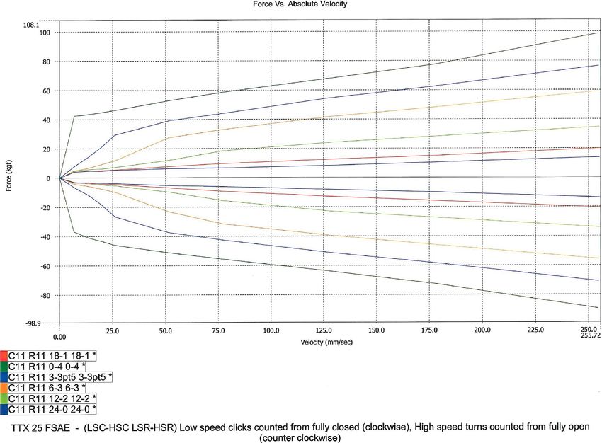
96                                                                     INGENIUS N.◦ 20, july-december of 2018

1. Introduction                                             2. Materials and methods

                                                          2.1. Study vehicle
Formula Student is a student competition organized
by the SAE (Society of Automotive Engineers) whose The vehicle used to study the suspension is a Formula
main objective is to promote the best training of young Student electric competition car, as shown in Figure
engineers [1], challenging university students to design, 1.
build and test the performance of a formula type vehi-
cle that successfully meets the tests stipulated in the
respective regulations [2], to then compete with other
students around the world.
    The technological advances and the level of compet-
itiveness generated by Formula Student have motivated
the UPS Racing Team of Universidad Politécnica Sale-
siana to develop two single-seater cars. The first one
was a combustion car for the 2014 competition in the
UK, while the second was an electric vehicle for the
UK Formula Student Electric competition in 2017.
    According to the results of last year [3], in the dy-       Figure 1. Formula Student electric single-seater
namic events the electric car has had problems with
some mechanical and electrical systems; among the              The dimensions of the car are shown in Table ??.
mechanical difficulties is the lack of adjustments in
the settings and the suspension damping, as well as a
                                                                Table 1. Dimensions of the electric single-seater
failure located in a member of the lower control arm
of the rear suspension.
                                                                         Especification                   Dimension
    Considering that the suspension plays a very impor-
                                                                      Front track width                      1200 mm
tant role in the performance of the vehicles in terms of
                                                                      Rear track width                       1180 mm
safety and comfort, there is a need to carry out studies
                                                                         Wheelbase                           1600 mm
of the suspension that allow for improvements either
                                                                      Weight with pilot                       345 kgf
in the development or in the design, so that the car
                                                                  Front weight distribution                     45%
can be competitive.
                                                                   Back weight distribution                     55%
    The main suspension design in competition is the              Height of center of gravity                 300 mm
deformable parallelogram (doublé A-arm or double
wishbone), which can have three forms of spring-
damper assembly activation, which are: direct, by
means of a push-rod, or pull rod [4]. These suspension 2.2. Suspension system characteristics
systems are simple in design, easy to adjust, resistant,
have good adaptability and can be light if they are The characteristics of the suspension system are shown
made with composite materials, which is why they in Table 2.
are widely used by Formula 1 and Formula Student
cars [5].                                                    Table 2. Suspension system characteristics

    The suspension must incorporate a good kinematic                 Specification                           Detail
design to keep the tire as perpendicular as possible           Type of suspension system
                                                                                                    Deformable parallelogram
to the pavement, to maintain optimal cushioning and                    (Front/rear)
                                                                    Activation system
adequate elasticity rates to keep the tire on the ground         spring - shock absorber                    Push-rod
at all times. In addition, the components must be resis-               (Front/rear)
tant so that they do not fail under static and dynamic                 Stabilizer bar
                                                                                                           Sprat type
                                                                       (Front/rear)
loads [6–9].                                                         Shock absorbers
                                                                                                         Ohlins TTX25
                                                                       (Front/rear)
    The objective of this work is to carry out the dy-            Rigidity of the spring
                                                                                                            150/200
namic and kinematic study of the suspension system                (front/front) (N/mm)
                                                             Total length of the boat/bounce
of the Formula Student electric vehicle, by means of                 suspension (mm)
                                                                                                             30/30
kinematic simulation programs and mathematical cal-                      Material              Carbon fiber and aluminum 7075 T6
                                                                           Tires                   19.5 x 7.5-10 (Hoosier), R25
culations, to determine the performance of the suspen-                     Rims                  7 in x 10 in (Braid), offset: +35
sion and to establish improvements or solutions to the
problems that arise during the study.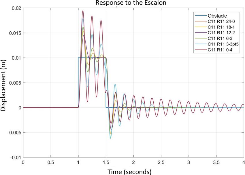
Arévalo et al. / Kinematic and dinamic study of the suspension system of an electric single seater competition
Formula Student                                                                                                        97

2.3. eometric parameters                                      dinates of the suspension connection points according
                                                              to [6, 7].
The coordinates of the connection points of each ele-
ment of the suspension are as shown in Table 3. The Table 4. Geometric parameters of the suspension system
connection points, in addition to allowing the defini-
tion of geometric parameters of the suspension, are                               Front        Rear
necessary for the kinematics simulation program and         Parameter
                                                                               suspension suspension
for the 3D calculation of the forces in the members of
                                                       Height of the balancing
the suspension.                                                                   44,84        70,02
                                                            center (mm)
                                                                  Angle of advance (°)           7               9
Table 3. Coordinates of the connection points of the sus-           Output angle (°)           8,13              0
pension’s elements                                                  Angle of fall (°)            0               0
                                                                 Mechanical Trail (mm)         28,32           70,02
            Front suspension           Rear suspension            Scrub radius (mm)            24,56             0
 Pts.   X(mm)    Y(mm)    Z(mm)    X(mm)    Y(mm)    Z(mm)         Anti-sinking / (%)
                                                                                                 0               0
  P1    1443,9     212    227,59     15       250    203,59           Anti-lifting
  P2     1732      212    227,59    335       250    203,59
  P3     1730      520    218,83   148,83     555      219
  P5    1446,6     256    377,59     15       290    347,59   An analysis is made of the results of the FSAE
  P4     1732      256    377,59    335       290        TIRE TEST CONSORTIUM [10], referring to the
                                                     347,59
  P5     1760      520    400,83   171,17     529      401
  P6     1710    480,74   244,78   148,83     513
                                                         Hoosier® tire 19.5 x 7.5-10, which is used in the study
                                                      241,8
  P8     1710    295,72   509,03   148,83     308        car. The analysis is carried out in order to determine
                                                     628,68
  P9     1790      520    218,83    220     549,14   259,83
                                                         the range of acceptable angles of fall, the behavior of
  P10    1750      190    227,59    220      258,5    234,2
  P11    1710     61,21   534,99   148,83    70,51       the tire and a prediction of the maximum forces it can
                                                     660,02
  P12    1710    238,98   534,99   148,83   245,98       withstand. Figure 3 shows that the maximum lateral
                                                      660,2
  P13    1760      520     310      160     541,98     310
  P14    1760      590     310      160       600
                                                         force is presented for an angle of fall of –1° to –1.3°,
                                                       310
  P15    1699    238,38   468,88   159,83   245,98       while the maximum longitudinal force is made for a
                                                     596,42
  P16    1721    238,38   468,88   137,83   245,98   596,42
                                                         fall of 0°. The tire does not suffer a sharp drop in grip
                                                         after reaching the maximum peak, so an effective fall
    Figure 2 shows the location of the connection points range of 1 to -3° can be set.
of the suspension elements.

                                                              Figure 3. Angle of fall at different lateral and longitudinal
                                                              forces, for a normal weight of 1000 N.

                                                              3. Results and kinematic analysis
                                                        Using Lotus Suspension Analisys, a kinematic analysis
                                                        of the suspension system is performed. The program
                                                        allows the user to know the behavior of the suspension
Figure 2. Location of the connection points of the sus- with the geometry established on various stages in the
pension elements.                                       track, such as bounce and rebound, roll and direction
                                                        turn [11]. The parameters that are analyzed are those
   Table 4 shows the geometric parameters based on that characterize the behavior of the suspension [12],
wheel dimensions, track gauge, wheelbase and the coor- such as: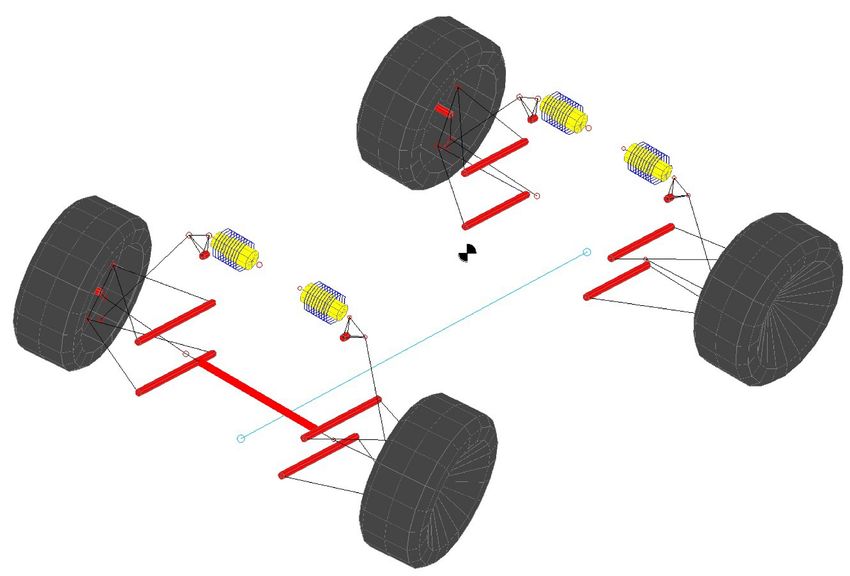
98                                                                     INGENIUS N.◦ 20, july-december of 2018

     • Balancing center

     • Angle of fall

     • Angle of advance

     • Toe (convergence/divergence)

    For the simulation, the dimensions of the car and
the coordinates of the connection points of each ele-
ment of the suspension are inserted into the program.
Lotus creates a three-dimensional model of the type
of suspension to be analyzed as shown in Figure 4.
                                                             Figure 5. Variations of the angle of fall with wheel bounce
                                                             and rebound.

                                                                 According to Figure 6, the forward advancing angle
                                                             becomes positive with the wheel bounce and negative
                                                             with the rebound, while the rear advancing angle has a
                                                             positive orientation in both bounce and rebound. The
                                                             angle of advance contributes to the gain of the angle
                                                             of fall during a turn. According to the results, during
                                                             curves the angle of advance will cause the external
                                                             wheel to have a negative fall gain and the fall of the
                                                             internal wheel to trend to be positive.
Figure 4. Simulated suspension system in Lotus Suspen-
sion Analysis.

     The elevation or bounce of the suspension in the
vertical direction is analyzed, which tries to simulate
the passage of the car over a bump or obstacle of 30
mm in height. For this analysis, only the right wheel
of the front and rear axle is considered, because the
left wheels display a similar behavior.
     Figure 5 shows that the front wheels in a bouncing
situation have a maximum negative fall gain of -1.13°,
and in rebound a maximum positive fall of 0.9°. The
rear wheels in the bouncing situation have a maximum
negative fall gain of -1.63°, and in rebound a maximum
positive fall of 1.41°. The behavior of the angle of fall
                                                             Figure 6. Variations of the angle of advance with wheel
is favorable according to [13], because when the vehicle
                                                             bounce and rebound.
passes through a curve, the most loaded wheel will
have a negative fall gain and the discharged wheel a
positive fall gain, improving the lateral grip and its
traction simultaneously. In order to achieve maximum
performance of the tire and reduce the positive angle of         Figure 7 shows that the maximum vertical travel of
fall, a static angle of fall for the front and rear wheels   the center of balance with the bounce and rebound is
of -1° and -1.5° respectively can be established. Hav-       80.344 mm and 86.4 mm for the front and rear suspen-
ing a static fall, wheels with maximum compression           sion respectively. The center of balance is maintained
approach a negative fall of -2.6°, staying within an ef-     at all times above the ground plane, something very
fective range of 1° and -3°, according to the analysis of    desirable according to [14]. The height of the center
the tires. According to the recommendation of Carroll        of balance to the center of gravity and the anti-roll
Smith [9], the static fall adjustment can be reduced         effect of the elastic elements allow the angle of roll of
by improving the grip of the tire in both curved and         the chassis to be 1° at a lateral acceleration of 1 G,
straight trajectories.                                       without considering the deformation of the tires.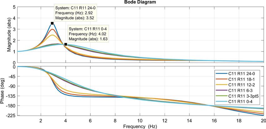
Arévalo et al. / Kinematic and dinamic study of the suspension system of an electric single seater competition
Formula Student                                                                                                        99

Figure 7. Variations of the height of the center of balance
with bounce and rebound of the wheel.                         Figure 9. Variations of the angle of fall with rolling of the
                                                              chassis.

    The maximum rear toe is 0.1393 degrees with wheel             Figure 10 shows that the rear and front swing cen-
rebound and maximum forward toe is 0.0328 degrees             ters have a lateral travel of 186.44 mm and 119.05 mm
with wheel bounce, as shown in Figure 8. A slightly           respectively, with a maximum rolling of the chassis
positive toe reduces rolling resistance and a negative        of 3°. Considering the effect in the reduction of the
toe improves maneuverability in curves, however, ex-          rolling of the elastic elements (springs and stabilizer
cessive toe increases tire wear. The low values are due       bar), as well as a lateral acceleration of 1 G; the chassis
to the fact that the bump steer effect is null, which has     will have 1° of roll, where the lateral migration of the
been achieved with a correct geometry of the steering         balancing center will be 63.57 mm/G and 40.25 mm/G
rods.                                                         in the front and rear suspension respectively.

                                                              Figure 10. Lateral movement of the center of rolling with
                                                              rolling of the chassis.
Figure 8. Toe variations with bounce and rebound of the        Figure 11 shows the behavior of the right front
wheel.                                                    wheel with the turn of the direction. When the wheel
                                                          is internal to the curve and with the maximum angle of
     The passage of the car through a curve is simulated, rotation has a negative fall of -2.75°. If the wheel is ex-
which causes the suspension to tilt due to centrifugal ternal to the curve, a positive fall of 5.33° is generated
acceleration. The lateral force is translated into a roll with the maximum turn.
angle of the chassis. According to Figure 9, when the
rolling of the chassis is positive the wheel is external 4. Results and dynamic analysis
to the curve and if it is negative the wheel is internal
to the curve. With a rolling of 3° of the chassis, the The calculations of the forces generated in the mem-
maximum angle of fall for the external and internal bers of the suspension system are performed when the
wheel of the front axle is 1.28 and -1.52 degrees respec- vehicle is subjected to different dynamic load scenar-
tively, while in the rear axle the maximum angle of ios. It is important to consider as many scenarios as
fall is 1,83° for the outer wheel and -2,01 for the inner possible because the forces generated will vary for each
wheel. Depending on the results, the wheels outside member depending on the load case. Five different
the curve have a negative fall gain, allowing for an load scenarios are established to which the vehicle is
improvement in tire grip.                                 subjected in a typical road environment [15].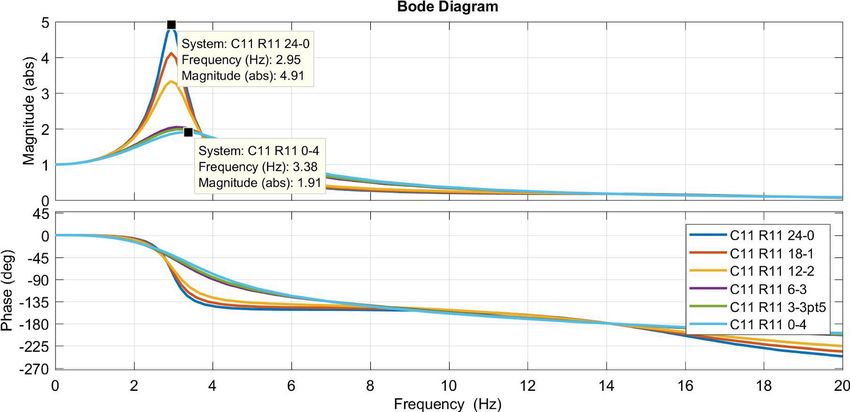
100                                                                  INGENIUS N.◦ 20, july-december of 2018

                                                                                          W × Ax × h
                                                                          W d = Wed +                            (5)
                                                                                              l
                                                                                          W × Ax × h
                                                                          W p = Wep −                            (6)
                                                                                              l
                                                            Where:
                                                               Ax = longitudinal acceleration (m/s2 )
                                                               vo = initial speed (m/s)
                                                               vf = final speed (m/s)
                                                               F t = tensile force (N)
                                                               W = weight of the vehicle (N)
                                                               l = wheelbase (m)
Figure 11. Variations of the angle of fall with the turn of    h = height of the center of gravity (m)
the direction.
                                                               µ = coefficient of adhesion
                                                               W ed = static weight on the front axle (N)
   • Linear acceleration                                       W ep = static weight on the rear axle (N)
                                                               W d = dynamic weight on the front axle (N)
   • Linear braking                                            W p = dynamic weight on the rear axle (N)
                                                               F f d = braking force on the front axle (N)
   • Passing through curve                                     F f p = braking force on the rear axle (N)
   • Acceleration in curve                                     b = distance from the axle posterior to the center of
                                                                    gravity (m)
   • Curved braking
                                                               The forces that are generated in the tire patch in
   • Passing through obstacle
                                                            the Y and Z directions due to the curve path as shown
    For each load scenario, the forces generated in the in Figure 13, are determined by equations 7, 8, 9.
referential system are calculated, X in longitudinal
direction to the vehicle, Z in perpendicular direction
to the ground and Y in the direction transverse to
the vehicle. The forces that are generated in the tire
patch in the X and Z directions due to acceleration
and braking as shown in Figure 12, are defined by
equations 1-6:

                                                            Figure 13. Forces present in the tire patch on the curve.

                                                                                         m × v2
Figure 12. Forces present in the tire patch during accel-                         Fl =                           (7)
eration and braking.                                                                     4×r
                                                                                  We   We × Ay × h
                            vf − vo                                       wre =      +                           (8)
                     Ax =                            (1)                          2        T
                               t
                                                                                          W × Ax × h
                           µ×W ×b                                         W p = Wep −                            (9)
                   Ft =      L
                                                     (2)                                      l
                             h
                          1− L ×µ                        Where:

                           W × Ax × h
                                                          m = mass of the vehicle (kg)
          F f p = µ × We −                           (3)   v = vehicle speed (m/s)
                               l
                                                           r = radius of curvature (m)

                           W × Ax × h                      Ay =lateral acceleration (m)
          F f d = µ × We −                           (4)   We = static weight on the axle (N)
                               l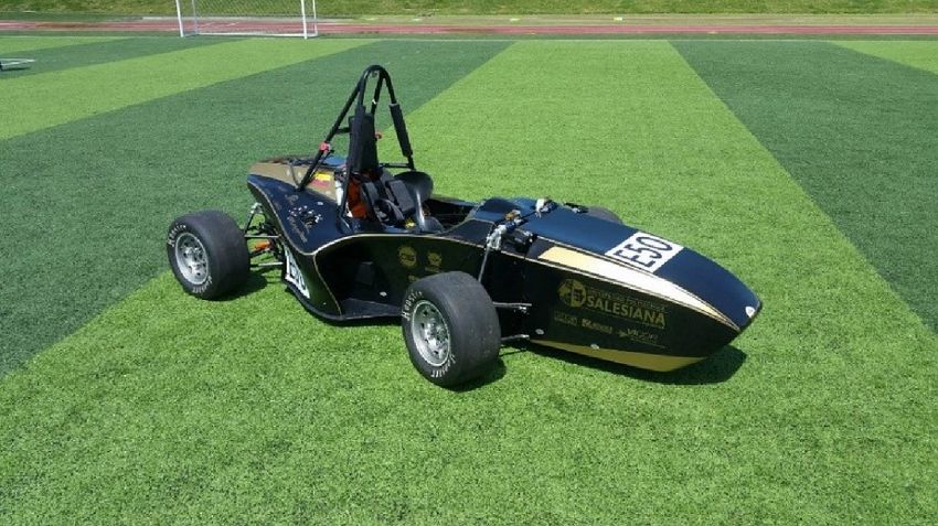
Arévalo et al. / Kinematic and dinamic study of the suspension system of an electric single seater competition
Formula Student 101
Wre = dynamic weight on the outer wheel (N) A system of vectors and matrices is used to deter-
Wri = dynamic weight on the inner wheel (N) mine how these forces are distributed along each of
T = track width (m) the suspension elements [16].
h = height of the center of gravity (m) With a balance of forces and moments with respect
The forces generated in the tire patch in the Z direc- to the X, Y and Z coordinate axes of the wheel center,
tion due to passing through an obstacle are determined six equations are determined. The system of equations
by equation 10: is solved by the following expression:
Feje = 0, 2maxis × az (10)
Where: [A]x = B
(11)
Faxis = force on the shaft (N) x = [A]−1 B
az =vertical acceleration (m/s2 )
maxis = mass of the axis (kg) x represents the unknown force in each of the sus-
With the established load scenarios, we proceed pension members.
to determine the forces that are generated in the sus-
pension members. In the front and rear suspension FP R
there are a total of six members, where two members FBCSF
are the upper control arm (BCS), two members of the FBCST
x= (12)
lower control arm (BCI), one of the push-rod (PR) FBCIF
and one of the coupling arm (BA). For this analysis FU CST
it is assumed that the load acts on the center of the FBA/BAD
wheel. The wheel center is considered to be the base of
the rigid body and point (0,0,0) as shown in Figures B represents the forces and moments in X, Y and Z
14 and 15. generated in the center of the tire patch and resolved
on the center of the wheel.
Fx
Fy
Fz
B=
(13)
M x
M y
Mz
The matrix A is determined by the unit vectors
obtained from the sum of forces and momentsin the X,
Figure 14. Free body diagram of the forces in the mem- Y and Z directions of each member. The force vector
bers of the front suspension.
→
−
(( F ) is equal to the product point between the unit
vector (u) and the magnitude of the force (|F |), as
−
→
shown in equation 15. The moment (M ) is equal to the
→
−
cross product between the force vector ( F ) and the
moment arm vector (→ −r ), as can be seen in equation
15.
→
−
F = |F | × →
−
u
−
→ → − → (14)
M = F ×− r
Figure 15. Free body diagram of the forces in the mem- −
→
bers of the rear suspension. M = |F | × →
−
u ×→
−
r (15)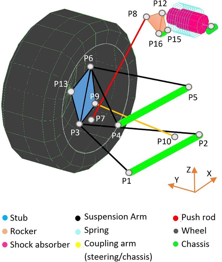
102 INGENIUS N.◦ 20, july-december of 2018
uP Rx uBCSF x uBCST x ...
uP Ry uBCSF y uBCST y ...
uP Rz uBCSF z uBCST z ...
[A] =
(uz ry − uy rz )P R
(uz ry − uy rz )BCSF (uz ry − uy rz )BCST ...
(uz rx − ux rz )P R (uz rx − ux rz )BCSF (uz rx − ux rz )BCST ...
(uy rx − ux ry )P R (uy rx − ux ry )BCSF (uy rx − ux ry )BCST ...
(16)
... uBCIF x uBCIT x uBAx
... uBCIF y uBCIT y uBAy
... uBCIF z uBCIT z uBAz
... (uz ry − uy rz )BCIF (uz ry − uy rz )BCIT (uz ry − uy rz )BA
... (uz rx − ux rz )BCIF (uz rx − ux rz )BCIT (uz rx − ux rz )BA
... (uy rx − ux ry )BCIF (uy rx − ux ry )BCIT (uy rx − ux ry )BA
Tables 5 and 6 show the maximum forces of tension the aluminum grafts and the carbon fiber tube is mea-
and compression in the members of the suspension sys- sured [17]. The graft is an aluminum element glued
tem, as a result of the different load scenarios. The with a high resistance adhesive to the carbon fiber tube,
maximum tensile forces in the members of the suspen- allowing the anchoring to the chassis or to the spindle
sion arms are –4313 N and –5131 N in the front and by means of ball joints. The tubes are of two external
rear respectively, and the maximum compression forces diameters, 18.1 mm and 21.3 mm with a thickness
are 4165 N and 5119 N. The front and rear push-rods of 1.15 mm. The larger diameter tube is used for the
work only in compression where the forces are 5358 N push-rod and the coupling arms. The smaller diameter
and 8544 N for the front and rear respectively. tube is used for the suspension arms.
Table 5. Results of the forces on the members of the front Table 7. Results of the compression and tensile tests of
suspension the members of the suspension
Load Forces on the members of Tube Traction Fuerza Compression
scenarios the front suspension diameter (mm) force (KN) force (KN)
FPR FBCSF FBCST FBCIF FBCIT FBAD 18,1 2,9 13,59
Acceleration (N) 487 109 82 –272 –178 –58 21,3 8,93 13,88
Braking (N) 1149 4162 –2726 –2021 3350 –2623
Curve (N) 1092 –1160 –1459 1063 957 825
Acceleration and According to the results of Table 7, it can be said
296 –1339 –1594 1508 1248 918
curve (N) that the members of the suspension arms could fail in
Braking and
2495 1013 4165 146 –4313 –1109 tension, since according to the tensile test, the maxi-
curve (N)
Step through mum joint force is 2.9 KN, and the maximum tension
5358 1203 906 –2990 –1954 –629
obstacle (N)
Maximum force in one member of the suspension arm is –5.13
force (N) 5358 4162 4165 –2290 –4313 –2623
KN. In the case of compression, the members are sub-
ject to buckling, therefore, it is necessary to perform a
calculation of critical buckling (Pcr ) and safety factor
Table 6. Results of the forces in the members of the rear (Fs ), defined by equations 18 and 19. The calculation
suspension will make it possible to more accurately predict a case
of compression failure [18].
Load Forces in the members of
scenarios the rear suspension
Cπ 2 El
FPR FBCSF FBCST FBCIF FBCIT FBAD Pcr = (17)
Acceleration (N) 1494 –3942 2874 4775 –5131 –776 l2
Brakimg (N) 754 2582 –1333 -2437 988 482
Curve (N) 2239 998 –2225 –155 1297 -625 Pcr
Acceleration and
2090 –3168 238 5119 –2503 52
Fs = (18)
curve (N) c
Braking and
curve (N)
956 –1772 -949 Where:
3553 –153 –268
Step through
8544 1646 1986 –2593 C = condition constant of articulated ends
–2915 521
obstacle (N)
Maximum P = axial force (N/m2 )
8544 –3942 2874 5119 –5131 776
force (N) E= modulus of material elasticity (N/m2 )
I= moment of inertia (m4 )
Compression and tensile tests are performed to de- l = length of the bar (m)
termine if the limbs support the maximum calculated According to the results of Table 8, the members of
loads. In the tensile test, the bond strength between the suspension arms, push-rod and coupling arm would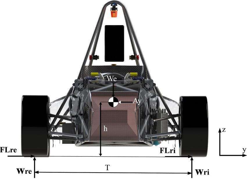
Arévalo et al. / Kinematic and dinamic study of the suspension system of an electric single seater competition
Formula Student                                                                                                          103

not fail due to buckling effects since, according to the degrees of freedom, which includes the elastic constant
calculation, they have safety factors greater than 2 and of the tire, as well as the non-suspended mass. The po-
support higher compression forces than 13 KN.                sition of the suspended mass is X1 , the non-suspended
                                                             mass is X2 and X0 serves to model the unevenness of
Table 8. Results of the calculation of critical buckling and the terrain.
safety factor of suspension members working by compres-
sion

       Tube            Buckling          Axial       Security
   diameter (mm)      critical (N)     force (N)      factor
         18,1           14 181,35         5119          2,77
         21,3           18 769,27         8544          2,19

    Since one of the most important tasks of the suspen-
sion system is to absorb the irregularities of the road
without losing traction in the tires, the vast majority
of cars are equipped with shock absorbers and springs
to fulfill this purpose. In this section, through a model
of 2 degrees of freedom of the suspension system of ¼
                                                            Figure 16. Full model of a quarter of a vehicle [11].
of the vehicle [19], the analysis of the frequencies of the
suspension is made, generating an interaction between
the road and the vehicle. Figure 16 shows the model          The transfer function of 2 degrees of freedom is
of the suspension of a quarter of the vehicle with 2 given by the following expression:

                  x2 (s)                           Rs · Kn · s · Ks · Kn
                         =                                                                                               (19)
                  x0 (s)   (m1 · s2 + Rs · s + Ks + Kn )(m2 · s2 + Rs · s + Ks ) − (Rs · s − Ks )2

   With the defined modeling, the necessary initial different damping coefficients for high and low speed
parameters are established to allow the study to be provided by the TTX 25 damper [20]. By means of
carried out, as shown in Table 9.                          equation 23 and the graph in Figure 17, the slopes or
                                                           damping coefficients for the different damper settings
Table 9. Parameters of the model of a quarter of a vehicle are determined as shown in Table 10.

                                       Front         Rear
           Parameter
                                    suspension    suspension
     m2: suspended mass (kg)           61,1           74,75
   Ks: suspension rigidity (N/m)     26 220,47      34 960,62
      Rs: suspension damping
                                      .......        .......
         coefficient (Ns/m)
      Kn: tire stiffness (N/m)      102 917,699    132 322,756
   m1: mass not suspended (kg)          10,9          13,25
         MR: motion ratio               1,3            1,4
    Kw: wheel stiffness (N/m)        15515,071      17837,051
   fm2: natural frequency of the
                                       2,36            2,3
       suspended mass (Hz).
   fm1: natural frequency of the
                                       16,62          16,81
      unsuspended mass (Hz)
       Ccr: critical damping
                                     2487,28        3233,274
         coefficient (Ns/m)

   The force developed by a shock absorber (Fa ) is                    Figure 17. Damping coefficients for different shock ab-
represented by the equation:                                           sorber settings [21]

                                                            To maximize the traction area, the lowest possible
                        Fd = Rs · vp                            (20)
                                                        transmissibility is required. The graphics of Figures 18
Where:                                                  and 19 show the response of the second-degree model of
   Rs = damping coefficient [Ns/m]                      the front and rear suspension. It can be seen that if the
   vp = speed on the piston of the shock absorber [m/s] damping factor is increased at low input frequencies,
                                                        the transmissibility is reduced to the maximum, which
   Using mathematical Matlab software, the trans- means that the tire will not lose traction. After the
missibility of the suspension system is analyzed at point of intersection, the low damping factors result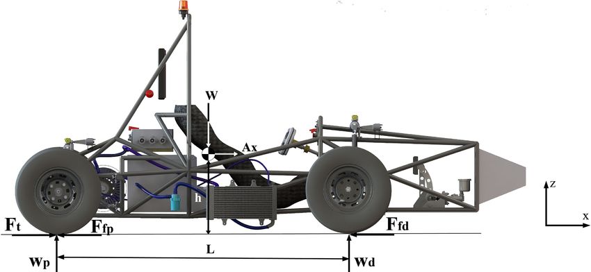
104 INGENIUS N.◦ 20, july-december of 2018
in a lower transmissibility, attenuating movement in
the chassis [22].
Table 10. Damping coefficients for different shock ab-
sorber settings
Low High
Adjustment of the speeds speeds Figure 19. Transmissibility of the second-degree model
shock absorber slope slope of the rear suspension.
[KN*s/m] [N*s/m]
C11 R11 0-4 52,788 2223
C11 R11 3-3pt5 11,77 1962
C11 R11 6-3 5,282 1831
C11 R11 12-2 2,354 882,9
C11 R11 18-1 3,678 689,1
C11 R11 24-0 3,678 567,5
Figure 20. Slope adjustment for high speeds and low
According to the transmissibility analysis, a high speeds. [23]
damping factor is necessary (ξ) at low speeds and a
low value for high speeds in the shock absorber. The
TTX25 shock absorber, for the front suspension, needs According to the analysis made, the use of double
a very close value of ξ = 0, 73, which is achieved with the compression damping factor for extension is de-
setting C11 R11 6-3 for low speed. For high speeds termined. In this way, it is possible to achieve a good
the setting C11 R11 24.0 provides un ξ = 0, 22. In the grip of the wheel, a lower transmissibility and bet-
rear suspension a value of ξ = 0, 68 is required, which ter maneuverability. The calibrations that meet these
is achieved with the C11 R11 0-4 setting for low speed. requirements are shown in Tables 11 and 12.
For high speeds the setting C11 R11 18.1 provides un
ξ = 0, 22. Table 11. Damping factor of the front suspension
Adjustment Compression Extension
of shock absorberr Low High Low High
speed speed speed speed
C11 R11 12-2 0,92 0,34 ...... ......
C11 R11 6-3 ...... ...... 2,08 0,72
Table 12. Factor de amortiguamiento de la suspensión
posterior
Adjustment Compression Extension
of shock absorberr Low High Low High
Figure 18. Transmissibility of the second-degree model speed speed speed speed
of the front suspension. C11 R11 12-2 0,72 0,27 ...... ......
C11 R11 6-3 ...... ...... 1,63 0,56
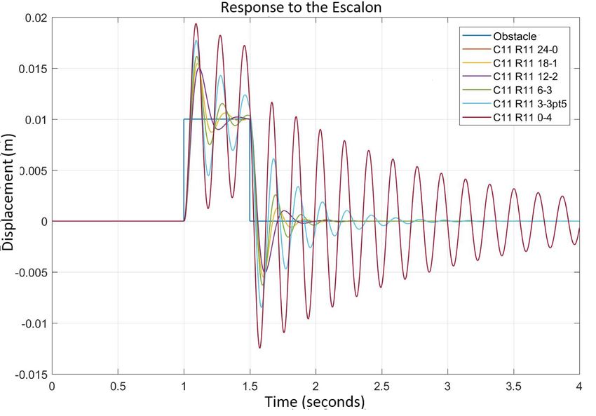
Figures 21 and 22 show the system response of
As the system moves both compression and exten- the front and rear suspension respectively in front of
sion, according to [23] it is better to have a damping a vertical displacement as input. It can be seen that
factor lower than compression and greater than exten- the calibrations of the low speed damping factor in
sion in relation to the desired value in order to avoid compression attenuate oscillations in the shortest time
resonance in the system (see Figure 20). possible with respect to other calibrations.Arévalo et al. / Kinematic and dinamic study of the suspension system of an electric single seater competition
Formula Student 105
that the suspension arms subjected to stress loads can
fail in critical cases, the problem is in the strength
of the joints between the aluminum grafts. With the
second-degree model of a quarter of a vehicle and with
the help of Matlab, a transmissibility analysis was car-
ried out that allowed defining the characteristics that
the shock absorber must have to guarantee maximum
contact area, which produces greater traction.
References
[1] IMechE. Formula student. Institution of
Mechanical Engineers. [Online]. Available:
Figure 21. Response of the front suspension system to a https://goo.gl/Mkjf9n
vertical displacement as input.
[2] S. International. (2017) Formula sae rules.
[Online]. Available: https://goo.gl/pSeNqe
[3] Formula Studente Germany. (2017) For-
mula student electric - world ranking list.
Mazur Events+Media. [Online]. Available:
https://goo.gl/2Q75AE
[4] A. Staniforth, Competition Car Suspension:
Design, Construction, Tuning, Haynes, Ed., 1999.
[Online]. Available: https://goo.gl/2jhg7s
[5] Rapid-Racer. (2016) Suspension. [Online]. Avail-
able: https://goo.gl/5Dpwjr
[6] W. F. Milliken and D. L. ;illiken, Race Car
Vehicle Dynamics, S. International, Ed., 1995.
Figure 22. Response of the rear suspension system to a [Online]. Available: https://goo.gl/iuhFqJ
vertical displacement as input.
[7] T. Pashley, How to Build Motorcycle-engined
Racing Cars, V. P. Ltd, Ed., 2008. [Online].
Available: https://goo.gl/XdxRGM
5. Conclusions
[8] M. Royce and S. Royec, Learn & Compete: A
This research helps to have a broader view of the sus- Primer for Formula SAE, Formula Student and
pension systems used by FSAE competition vehicles. Forumula Hybrid Teams, R. Graphic, Ed., 2012.
With the study of the kinematics, the behavior of the [Online]. Available: https://goo.gl/9rxtrG
suspension of the car was determined under different [9] C. Smith, Tune to Win, C. S. Consulting, Ed.,
scenarios on the track, such as passing through a curve 1978. [Online]. Available: https://goo.gl/KaTkxq
or an obstacle. Depending on the results, it can be
said that the configuration provided for the single- [10] Milliken Research. (2018) Formula sae tire test
seater’s suspension allows a good directional control of consortium. Milliken Research Associates Incorpo-
the vehicle (null bump steer effect) and an adequate rated. [Online]. Available: https://goo.gl/ErGrP5
negative fall gain of the wheel with the travel of the
[11] G. P. Pillajo Quijia, “Estudio cinemático del
suspension or rolling of the chassis, giving a good lat-
comportamiento de la suspensión de un prototipo
eral grip to the tires. However, with the turn of the
de formula sae student eléctrico del equipo upm
steering there is a gain of excessive positive fall in the
racing,” Master’s thesis, Universidad Politécnica
front wheels, which would affect the lateral grip in very
de Madrid. España, 2012. [Online]. Available:
tight corners. With the appropriate adjustments in the
https://goo.gl/aTb5mt
angles of advance, exit, static fall and convergence,
the required or optimal conditions of vehicle stability [12] P. De la fuente aguilera, “Análisis de la suspensión
and steering could be ensured, allowing greater ac- del vehículo monoplaza eléctrico UPM-03e del
celerations, better braking and faster cornering steps. equipo UPM racing,” Universidad Politécnica
According to the study of the forces in the members of de Madrid. España., 2016. [Online]. Available:
the suspension with dynamic loads, it was determined https://goo.gl/PvvCV3106 INGENIUS N.◦ 20, july-december of 2018
[13] S. Juvanteny Gimenez, “Estudio y diseño del sis- M. Mc Graw-HILL, Ed., 2012. [Online]. Available:
tema de suspensión para un prototipo de fórmula https://goo.gl/dumukn
sae,” Tesis de grado. Universidad Politécnica
de Cataluña. España, 2015. [Online]. Available: [19] F. Aparicio Izquierdo, Teoría de los vehíulos
https://goo.gl/q93zhh automóviles, E. T. S. d. I. I. Universidad Politéc-
nica de Madrid, Ed., 1995. [Online]. Available:
[14] E. I. Efler herranz, “Diseño de la suspensión https://goo.gl/M2EHoy
trasera de un vehículo formula student,” Tesis de
grado. Universidad Politécnica de Madrid. España, [20] J. Hurel, E. Teran, F. Flores, and B. Flores,
2016. [Online]. Available: https://goo.gl/YkgNnv “Modelo físico y matemático del sistema de
suspensión de un cuarto de vehículo,” in 15th
[15] E. D. Flickinger, “Design and analysis of formula LACCEI International Multi-Conference for En-
sae car suspension members,” Master’s thesis, gineering, Education, and Technology. USA, 2017.
California State University, Northridge. EEUU, [Online]. Available: https://goo.gl/7yrFEK
2014. [Online]. Available: https://goo.gl/tcUw5g
[21] ´’OHLINS. (2017) Ttx25 mkii,. ´’OHLINS. Ad-
[16] L. Borg, “An approach to using finite element vanced Suspension Technology. [Online]. Available:
models to predict suspension member loads in https://goo.gl/Kra2dB
a formula sae vehicle,” Master’s thesis, Virginia
Polytechnic Institute and State University. USA, [22] A. Espejel Arroyo, “Rediseño de un sistema
2009. [Online]. Available: https://goo.gl/i8bV4B de suspensión para un auto de competencia
mediante adams/car y matlab,” Tesis de grado.
[17] A. C. Cobi, “Design of a carbon fiber suspension Universidad Nacional Autónoma de México, 2015.
system for fsae applications,” Bachelor thesis. [Online]. Available: https://goo.gl/sTxBg9
Massachusetts Institute of Technology. USA,
2012. [Online]. Available: https://goo.gl/h1tQU3 [23] M. Giariffa and S. Brisson, “Tech tip: Spring &
dampers, episode four. a new understanding,” OP-
[18] R. G. Budynas and J. K. Nisbett, Diseño TIMUMG. Vehicle dynamics solutions, Tech. Rep.,
en ingeniería mecánica de Shigley, 9th ed., 2017. [Online]. Available: https://goo.gl/kVkg6oYou can also read