SPATIAL INFORMATION COMPREHENSIVE WELL-BEING COMPOSITE INDICATORS: AN ILLUSTRATION ON ITALIAN - SIEDS
←
→
Page content transcription
If your browser does not render page correctly, please read the page content below
Rivista Italiana di Economia Demografia e Statistica            Volume LXXV n. 1 Gennaio-Marzo 2021

     SPATIAL INFORMATION COMPREHENSIVE WELL-BEING
    COMPOSITE INDICATORS: AN ILLUSTRATION ON ITALIAN
                   VARESE PROVINCE1

                               Carlotta Montorsi, Chiara Gigliarano

1. Introduction

     In recent years, the concept of well-being and its measurement has been at the
forefront of the European research topic debates (Stiglitz et al., 2009). However,
despite some great advancements, a unique definition of well-being has not been
provided yet (Fiorillo et al., 2017). The well-being is thought as a multidimensional
phenomenon that mirrors the values and preferences of a society and its citizens.
Hence, its effective and faithful description requires relying on a set (or dashboard)
of relevant indicators (Hall et al., 2010). On the other hand, to enhance practicability,
the complex information enclosed in such a dashboard of indicators must be
synthesized through the construction of composite indicators (European
Commission, 2008).
     Within the Italian framework, the first project contextualized to this debate is
the “Equitable and Sustainable Well-being (Bes)”, jointly proposed in March 2013
by the National Council for Economics and Labor (Cnel) and the Italian National
Institute of Statistic (Istat, 2018). In 2016, to complement this project with one more
focused on the local level (NUTS3), a new project was started on “Well-being and
planning measure at the municipal level (“Misure di benessere e programmazione a
livello comunale”), coordinated by Istat, National Association of Italian
municipalities (ANCI) and Union of Italian Provinces. The project aims to provide
an integrated and harmonized data-set and information systems with a high local
detail and to support local authorities in policymaking. The resulting dataset “A
Misura di Comune” comes from an integration of different data sources, such as
administrative archives or statistical surveys, which share the characteristic of being
total and not sample sources.

1
  The authors gratefully acknowledge funding support from Fondazione Giovanni Valcavi per l’Università degli
Studi dell’Insubria.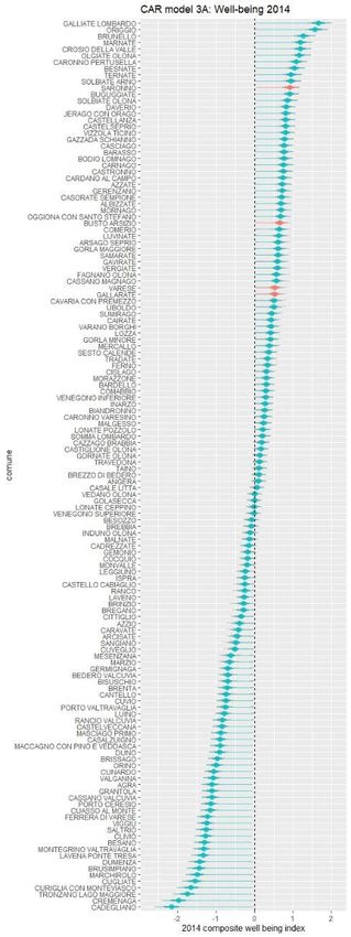
30                                                                    Volume LXXV n. 1 Gennaio-Marzo 2021

     The main differential aspect of this data-set with respect to the others elaborated
by Istat - “Bes” and “UrBes”- is the presence of particularly meaningful well-being
domains, such as “Population and family” and “Mobility and Infrastructure”, for the
use of their indicators in the “Single Programming document of local authorities”.
     This paper exploits the “A Misura di Comune” dataset2 for assessing the well-
being of the Varese province by constructing composite indicators that synthesize,
on a statistical basis, the atomic indicators information. We implement Bayesian
factor analysis for spatially correlated data. Factor analysis for constructing
composite indicators on BES dataset has already been proposed, for example in
Chelli et al. (2015) and Ciommi et al. (2017). However, to the best of our
knowledge, this is the first attempt to construct well-being composites indicators
inclusive of spatial information in the underlying statistical model.

2. Methodology

     The “A Misura di Comune” dataset is constituted by 50 atomic indicators, which
are grouped into 10 macro-domains. Data are collected for four years, from 2014 to
2017, in all Italian municipalities.
     The state of the art of aggregation methods entails a broad list of different
approaches, form the simpler linear aggregation to more constructed ones.
Constructed empirical indices, such as AMPI or GAMPI, are built on non-
substitutable and non-compensatory indicators and allow for comparison across
space (Mazziotta and Pareto, 2013). Nonetheless, they are based on several structural
assumptions (Ciommi et al., 2017). For example, no adjustment is made for
differential precision of the atomic indicators across local units that may have
different population sizes. Moreover, it is usually assumed that for a specific area,
information about well-being depends exclusively on variables from that area, and
not on variables from neighboring areas. And finally, the traditional indices lack a
posterior measure of uncertainty. This last feature can be problematic, for example,
if decisions about policies or resource allocation are based on cutoff values or
percentile of the index.
     Hence, we try to move forward these shortcomings exploiting the methodology
introduced in Hogan et al. (2004). We treat the “A Misura di Comune” atomic
indicators as manifest variables while the well-being is the underlying latent factor.
Hence, the well-being is defined as the posterior expectation of the latent factor given
the manifest variables and the model parameters. Therefore, under the assumption

2
    The dataset is available at http://amisuradicomune.istat.it/aMisuraDiComune/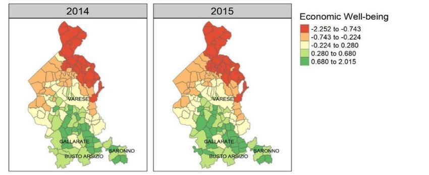
Rivista Italiana di Economia Demografia e Statistica                               31

that adjacent areas have similar socioeconomic characteristics, we introduce spatial
dependencies among the latent well-being variable of each municipality.
     Given the presence of missing values, we have restricted our analysis to two
years, 2014 and 2015. Moreover, we excluded from the analysis the indicators
related to the domain “Population and family”, since they are not strictly related to
well-being. Our analysis hence is based on 32 atomic indicators and focuses on the
139 Varese province municipalities.
     Our prior hypothesis is that neighboring municipalities share information on
socio-economic development levels. Hence, accounting for their spatial information
should increase the accuracy of our estimates. Therefore, before constructing the
statistical model, we tested for spatial autocorrelation in the atomic indicators
through the Global Moran I test (Moran, 1950), which provided significant results
for almost all the indicators.
     For municipality , with = 1, … , and = 139, let              denotes the atomic
indicator       in municipality , where        = 1, … , , and = 32. Hence           =
( , … , ) is the well-being profile of municipality . The general latent factor
model assumes for each area a L dimensional ( < ) latent variable δ =
(δ , … , δ ) , that fully characterizes socio-economic characteristics, which in turn
manifest themselves through . We assume = 1, hence reducing the model to one
latent factor for each municipality and we represent the model in a hierarchical form.
     At the first level we have:

                    Y ∣ μ , δ , Σ ∼ Multivariate-Normal(μ + λδ , Σ),

where μ is        × 1 mean vector, λ is a × 1 vector of factor loading's and Σ =
diag(σ , … , σ ) is a diagonal matrix measuring residual variation in . Assuming
Σ diagonal implies independence among the elements of conditionally on δ .
    Spatial autocorrelation is introduced at a second level. Let δ = (δ , … , δ ) the
municipalities’ latent indexes vector. Thus, it is assumed:

                             δ ∼ Multivariate-Normal(0 , Ψ),

where Ψ is a ×         spatial variance-covariance matrix having 1's on the diagonal
and ψ =           δ , δ on the off-diagonal. When Ψ = the model assumes spatial
independence. The well-being composite index for municipality is summarized by
the conditional distribution of the latent factor δ given and μ, λ, Σ. Hence the
posterior distribution of vector δ is a Multivariate normal distribution: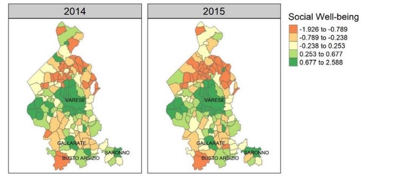
32                                                                Volume LXXV n. 1 Gennaio-Marzo 2021

                        ( δ ∣ , μ, λ, Σ ) ∼ Multivariate-Normal( , ),

                 where       = {Ψ + Λ Σ         Λ}     and        = Λ Σ       ( − μ).

      We have chosen a conditional parametrization of the spatial variance-covariance
matrix Ψ, through conditional auto-regressive specifications of spatial dependency.
The more general structures are the Gaussian CAR models (Besag J.,1974; Sun et
al., 1999). Generally, these models require to construct a set ℛ ,denoting the set of
indices δ for areas that are neighbors of the area . Then, they assume that:

                            δ ∣ {δ : ∈ ℛ } ∼             ∑   ∈ℛ    β δ ,     ,

so that
                      (δ , … , δ ) ∼ Multivariate-Normal(0 , ν                    ),

where is        × matrix with {α , … , α } along the diagonal and −α β on the
off-diagonal, provided that is symmetric and positive definite (Sun et al., 1999).
In order to ensure these conditions to hold one must constrain one or more
parameters, but the constraints are model specific.
     According to how we have defined the ℛ and β , different CAR models are
specified. For this analysis we have defined:     = ( ∈ ℛ ), which is the indicator
function that area is a neighbor of area , β = ω , α = 1 and ν = 1; then =
   − ω , where is an adjacency (weight) matrix with         = 0 and indicators     =
   . One necessary condition for         to be positive definite is that the ordered
eigenvalues ξ , … , ξ of have to satisfy: ξ < ω < ξ .
     Finally, a characteristic of the Bayesian framework is the introduction of prior
distributions on all the model's parameters. In our model we have set: λ ∼
Normal( , ) (λ > 0); σ ∼ Inverse-Gamma(α/2, β/2); μ ∼ Normal 0, .
     The scope of prior distributions is to include subjective opinions on the
parameters of interest. However, we let the data “speak for them-self” and choose
uninformative priors with = 0, = 10000, α = 1/1000, β = 1/1000, = 1000.
     The model is estimated through a Gibbs sampling that includes Metropolis
Hasting steps for the spatial parameter ω.3

3
  We have written the sampling algorithm in the R software and made it available in GitHub through the link
https://github.com/CarlottaMnt/Bayesian-factor-analysis-sampler.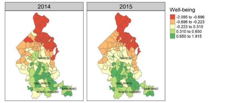
Rivista Italiana di Economia Demografia e Statistica                                                      33

3. Results

      Following this methodology, we have first computed a uni-dimensional overall
well-being composite indicator which synthesizes, for each municipality, the 32 “A
Misura di Comune” atomic indicators.
      In Table 1 we report the factor loadings' distributions, which represent the
covariances among the “A Misura di Comune” atomic indicators and the composite
indicator (latent variable). Factor loadings with negative sign impact negatively the
latent well-being, such that an increase in the corresponding atomic indicator leads
to a decrease in the overall well-being. On the other hand, factor loadings with a
positive sign would raise the value of the overall well-being. When the estimated
factor loading is around zero all along its distribution, we consider the associated
indicator meaningless for the well-being.
      The main contributor with a positive impact on the composite indicator is the
“Gross Income per capita” while the one with the greater negative impact is
“Household with gross income less than the social allowance benefit”. Having zero
impact are the “Self-containment index”4 and the “Leakage of drinking water”.
      Figure 1 illustrates the estimate of the well-being composite indicator for the
Varese municipalities in 2014 and 2015. For each municipality, the graph reports the
mean value of the composite indicator and its posterior 95% credibility intervals. We
have highlighted in red the most populated municipalities, i.e. Varese, Gallarate,
Busto Arsizio and Saronno. Among the two years considered, the municipalities’
rank in term of composite indicator slightly changes, while the polarization among
municipalities does not change significantly.
      Finally, the maps in Figure 2 report the spatial distribution of the composite
indicator's mean across the Varese municipalities. The above-average values are in
green while below-average values are in red. We notice clusterization in the well-
being phenomenon, which is discriminated among northern and southern
municipalities, whereas the first appreciate the lowest level of well-being and the
latter are better off. This result is maintained throughout the two years considered.
      Next, we proceed with our well-being assessment by constructing a composite
indicator for each of the three, non-fungible, sustainable development domains:
social well-being, economic well-being and environmental well-being (Ciommi et
al., 2020). This will clarify the contribution each domain provides on the overall
well-being and the relative importance of the atomic indicators with respect to the
specific well-being composite indicator they interact with. It may be that, when the
number of atomic indicators in each domain is too little, the uncertainty of the
composite indicator as well in the factor loading's estimates increases.
4
 It represents the ratio among the monetary flows from those who work within the municipal boundaries and the
overall monetary flows generated overall in the municipality.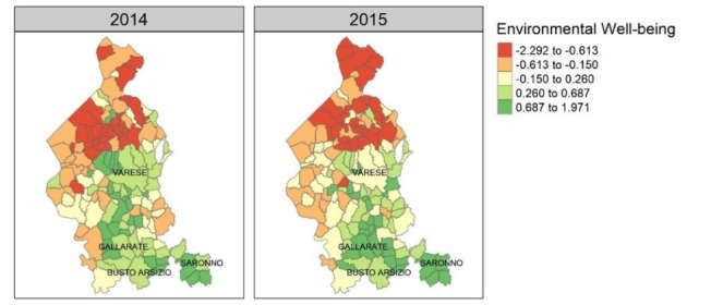
34                                                        Volume LXXV n. 1 Gennaio-Marzo 2021

     As a first result, Table 2 to Table 4 report the factor loading's distribution in the
four domains.

Table 1 - Summary of the factor loadings' distribution for each “A misura di comune”
indicators, year 2014.
     Indicator                                           Mean      5%      50%      95%
     Circulating polluting vehicles                       -2.70    -7.46    -0.67    -0.51
     Children in municipal childcare services              0.83     0.05     0.21     2.27
     Household low labour intensity                       -4.23   -12.28    -1.03    -0.85
     Soil consumption                                      3.53     0.67     0.84   11.65
     IRPEF taxpayers with total income < 10.000           -4.38   -11.52   -1.00     -0.83
     Local units’ density                                  3.25     0.59     0.75     9.86
     High school graduates (25-64)                         2.47     0.48     0.63     6.98
     Leakage of drinking water                             0.40    -0.06     0.09     0.67
     Gross income differences                              4.41     0.83     1.00   12.74
     Women and political representation - City Council    -0.20    -0.20     0.01     0.20
     Women and decision-making - Municipal council         0.92     0.07     0.22     1.99
     Mean age local administrator                         -0.84    -2.17    -0.19    -0.04
     Mean age municipal councillors                       -0.49    -0.73    -0.09     0.07
     Household with gross income less then social
                                                          -4.39   -12.96   -1.01    -0.84
      allowance benefit
     Single-income households with children (age < 6)     -2.56    -7.20   -0.58    -0.43
     Neet                                                 -4.08   -12.42   -0.99    -0.81
     Attraction Index                                      2.25     0.37    0.52     6.18
     Self-containment index                                0.12    -0.18    0.02     0.21
     Harmfulness of road accidents                        -1.26    -3.31   -0.30    -0.15
     Mortality index of road accidents                     0.29    -0.01    0.15     0.95
     Employed (20-64)                                      4.58     0.85    1.02    13.37
     Not stable employed                                  -1.53    -3.27   -0.31    -0.16
     Graduates (30-34)                                     2.36     0.40    0.56     6.66
     Museum, galleries, monuments                         -1.50    -4.28   -0.39    -0.23
     Electoral participation                               2.73     0.48    0.63     8.00
     Separate collection of municipal waste                1.06     0.17    0.33     3.76
     Gross per capita income                               4.33     0.84    1.02    13.02
     Production specialization in high-tech sectors        1.95     0.34    0.49     5.96
     Rate of entrepreneurship                              2.86     0.56    0.73     8.73
     Number of road accidents                              0.78     0.02    0.18     1.68
     Jobs' transformation from not stable to stable        1.09     0.10    0.26     2.81
     Visitors to museum, galleries, monuments             -0.62    -1.65   -0.14     0.01
Source: our elaboration on “A misura di comune” data.
Rivista Italiana di Economia Demografia e Statistica 35
Figure 1 Overall well-being indicator estimate and its 95% credibility interval for 2014
and 2015.
Source: our elaboration on “A Misura di Comune" data.36 Volume LXXV n. 1 Gennaio-Marzo 2021
Table 2 Social well-being: factor loadings' distribution, year 2014.
Indicator Mean 5% 50% 95%
Children in municipal childcare services -0.31 -0.22 -0.07 -0.01
High school graduates (25-64) 0.85 0.45 0.64 0.85
Women and political representation - City Council 0.55 0.10 0.29 0.50
Women decision-making - Municipal council 0.57 0.15 0.33 0.52
Mean age local administrator -0.60 -0.67 -0.45 -0.24
Mean age municipal councillors -0.26 -1.09 -0.26 0.53
Neet -0.56 -0.65 -0.45 -0.25
Harmfulness of road accidents -0.33 -0.45 -0.26 -0.08
Mortality index of road accidents -0.37 -0.32 -0.12 0.06
Graduates (30-34) 0.85 0.48 0.65 0.86
Museum, galleries and monuments 0.12 -0.25 -0.04 0.17
Number of road accidents -0.56 -0.33 -0.13 0.05
Visitors to museum, galleries and monuments 0.26 -0.17 0.01 0.21
Source: our elaboration on “A misura di comune" data
Table 3 Economic well-being: factor loadings' distribution, year 2014.
Indicator Mean 5% 50% 95%
Household low labour intensity -6.84 -44.49 -1.05 -0.89
IRPEF taxpayers with total income < 10.000 euros -6.72 -45.48 -1.03 -0.89
Local unit density 4.44 0.57 0.68 28.21
Gross income differences 6.51 0.84 0.99 44.25
Household with gross income < social allowance -6.66 -44.62 -1.05 -0.89
Single-income households with children (age < 6) -4.15 -27.65 -0.63 -0.51
Attraction Index 3.25 0.40 0.51 20.70
Self-containment index -0.44 -1.53 -0.06 0.03
Employed (20-64) 6.78 0.89 1.04 45.30
Not stable employed -2.21 -14.35 -0.35 -0.26
Electoral participation- municipal elections 3.99 0.54 0.65 28.30
Gross per capita income 6.40 0.84 0.99 42.29
Production specialization in high-tech sectors 3.27 0.40 0.50 22.16
Rate of entrepreneurship 0.63 0.47 0.63 0.79
Jobs transformation from not stable to stable 1.72 0.19 0.28 10.97
Source: our elaboration on “A misura di Comune" data
Table 4 Environmental well-being: factor loadings' distribution, year 2014.
Indicator Mean 5% 50% 95%
Circulating polluting vehicles -0.90 -0.84 -0.66 -0.46
Soil consumption 0.98 0.49 0.65 0.83
Leakage of drinking water 0.10 0.04 0.21 0.40
Separate collection of municipal waste 0.05 0.05 0.26 0.44
Source: our elaboration on “A misura di Comune" data
The leading domain is “economic well-being” (Table 3), where all the factors'
loadings, in absolute value, are far from being zero. In this domain, the indicatorsRivista Italiana di Economia Demografia e Statistica 37
driving the composite indicator to greater positive values are “Gross per capita
income” and “Employed (20-64)”. Table 2 reports the social well-being indicators'
factor loadings. With greater positive impact on the social well-being, despite being
small and near zero, are “High school graduates” and “Graduates (25-64)”, revealing
the importance of education in boosting the estimated well-being. Lastly, the
environmental well-being (Table 4) is mainly explained by “Soil consumption”,
which is the ratio among the soil consumed and the overall municipal soil, and
“Circulating vehicles with standard emissions lower than euro 4”, that points out the
negative role played by motor vehicles on air pollution.
Figure 2 Overall well-being indicator's spatial distribution in Varese province.
Figure 3 Social composite indicator's spatial distribution in Varese province.
Finally, we move directly to the spatial distribution of the composite indicators
across the Varese province. Figures from 3 to 5 map respectively the mean of the
composite indicator distribution for social well-being, economic well-being and
environmental well-being. The social well-being composite indicator interestingly
shrinks from 2014 to 2015: the worse off municipalities, despite remaining below
the average, increase their social well-being, indeed they become “clearer”, while38 Volume LXXV n. 1 Gennaio-Marzo 2021
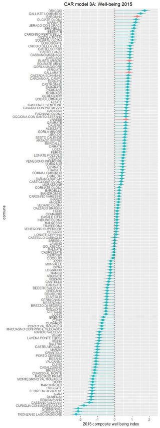
the better off municipalities slightly reduce their social well-being. The spatial
distribution for the economic well-being composite indicator detects the presence of
three separated groups, from the Southern to the Northern municipalities, with high,
medium and low economic well-being. This figure looks like Figure 1, corroborating
the greater importance of economic well-being in driving the overall well-being.
Finally, the environmental well-being spatial distribution also highlights differences
among municipalities in the North and in the South, with the latter performing better
Figure 4 Economic composite indicator's spatial distribution in Varese province.
Figure 5 Environmental composite indicator's spatial distribution in Varese province.
4. Concluding remarks
We have constructed well-being composite indicators by adopting a Bayesian
latent variable approach which includes spatial information. From the overall well-
being assessment on the Varese province, we have estimated heterogeneous well-
being levels across the province's municipalities. Notably, when considering all the
“A Misura di Comune” atomic indicators, the resulting composite indicator isRivista Italiana di Economia Demografia e Statistica 39
clustered among Northern and Southern municipalities, where the former enjoys, on
average, a lower well-being level with respect to the latter.
Next, we have analyzed the well-being within each of the three sustainable
development domains. We have highlighted the greater importance of economic
well-being in driving the overall municipalities' well-being. Within this domain, the
leading indicators are related to income and occupational levels.
Given the severe presence of missing values, our analysis focuses only on two
years, 2014 and 2015. However, as soon as updated data becomes available, future
research will consider the inclusion of temporal information within the model.
References
BESAG J. 1974. Spatial interaction and the statistical analysis of lattice systems,
Journal of the Royal Statistical Society: Series B, Vol. 36, No. 2, pp. 192-225.
CHELLI F.M., CIOMMI M., EMILI A., GIGLIARANO C., TARALLI S. 2015.
Comparing equitable and sustainable well-being (Bes) across the Italian provinces:
a factor analysis-based approach, Rivista Italiana di Economia Demografia e
Statistica, Vol. 69, pp. 61-72.
CIOMMI M., GIGLIARANO C., EMILI A., TARALLI S., CHELLI F.M. 2017.
A new class of composite indicators for measuring well-being at the local level:
An application to the equitable and sustainable well-being (Bes) of the Italian
provinces, Ecological indicators, Vol. 76, pp. 281-296.
CIOMMI M., GIGLIARANO C., TARALLI S., CHELLI F.M. 2017. The equitable
and sustainable well-being at local level: A first attempt of time series aggregation,
Rivista Italiana di Economia Demografia e Statistica, Vol. 71, No. 4, pp. 131-142.
CIOMMI M., GIGLIARANO C., CHELLI F.M., GALLEGATI M. 2020. It is the
total that does [not] make the sum: nature, economy and society in the Equitable
and Sustainable Well-Being of the Italian Provinces, Social Indicators Research,
https://doi.org/10.1007/s11205-020-02331-w.
EUROPEAN COMMISSION, 2008. Handbook on constructing composite
indicators: methodology and user guide. OECD publishing.
FIORILLO F., MUSCILLO C., TARALLI S. 2017. Misure di benessere dei
territori e programmazione strategica: il livello comunale, Economia pubblica,
Vol. 1, pp. 61-96.
HALL J., GIOVANNINI E., MORRONE A., RANUZZI G. 2010. A framework to
measure the progress of societies, OECD Statistics Working Papers 05, OECD
Publishing, Paris, https://doi.org/10.1787/5km4k7mnrkzw-en.
HOGAN J. W., TCHERNIS R. 2004. Bayesian factor analysis for spatially
correlated data, with application to summarizing material deprivation from census40 Volume LXXV n. 1 Gennaio-Marzo 2021
data, Journal of the American Statistical Association, Vol. 99, No. 466, pp. 314-
324.
ISTAT 2018. Il benessere equo e sostenibile in Italia. Roma: Istat.
MAZZIOTTA M., PARETO A. 2013. A non-compensatory composite index for
measuring well-being over time, Cogito, Multidisciplinary Research Journal, Vol.
5, No. 4, pp. 93-104.
MORAN P.A. 1950. Notes on continuous stochastic phenomena, Biometrika, Vol.
37, No.1/2, pp. 17-23.
STIGLITZ J.E., SEN A., FITOUSSI J.P. 2009. Report by the commission on the
measurement of economic performance and social progress. Paris: Commission on
the Measurement of Economic Performance and Social Progress
SUN D., TSUTAKAWA K., SPECKMAN P.L. 1999. Posterior distribution of
hierarchical models using car(1) distributions, Biometrika, Vol. 86, pp. 341-350.
SUMMARY
Spatial information comprehensive well-being composite indicators: an
illustration on Italian Varese province
This analysis bears upon the European “Beyond GDP initiative”, which promotes multi-
dimensional approaches going beyond the traditional and uni-dimensional GDP
macroeconomic indicator to monitor the living condition and the well-being of a territory.
We assess the well-being within the Varese province by applying factor analysis with
integration of spatial information in a Bayesian framework. To summarize the large number
of indicators within the 10 domains that constitutes “A misura di comune” dataset we
construct four composite indicators for each Varese municipality. The first is comprehensive
of all the “A misura di comune” indicators but not the one related to the Population and
Family domain. The last three composite indicators assess the municipalities in term of their
social, economic and environmental well-being. We highlight differentials across Northern
and Southern municipalities in all the well-being domains, with the former performing
usually better. We also identify in the economic domain the leading well-being domain, that
drives the overall wealth to higher values.
_______________________________
Carlotta MONTORSI, Università dell’Insubria, carlotta.montorsi@uninsubria.it
Chiara GIGLIARANO, Università dell’Insubria, chiara.gigliarano@uninsubria.itYou can also read