Statistics and probability for advocates: Understanding the use of statistical evidence in courts and tribunals - rss.org.uk
←
→
Page content transcription
If your browser does not render page correctly, please read the page content below

Statistics and probability for advocates: Understanding the use of statistical evidence in courts and tribunals
©2017 – The Council of the Inns of Court (COIC) and the Royal Statistical Society (RSS) 2
INTRODUCTION
  An introductory guide for advocates produced by the Royal Statistical Society
  and the Inns of Court College of Advocacy as part of the ICCA’s project:
  ‘Promoting Reliability in the Submission and Handling of Expert Evidence’.

 ‘The Inns of Court College of Advocacy is proud to have
 collaborated with the Royal Statistical Society over the
 production of this booklet. On the College’s side it forms
 a major building block in the development of the
 training of advocates in the effective understanding,
 presentation and challenging of expert evidence in
 court. Experts in every type of discipline, appearing in
 every type of court and tribunal, habitually base their
 evidence on statistical data. A proper understanding of
 the way in which statistics can be used – and abused –
 is an essential tool for every advocate.’
                                      Derek Wood CBE QC, Chair of the Governors of the ICCA

 ‘More and more fields of expertise are using data. So
 expert evidence, whether in pre-trial or in court, will
 increasingly include a statistical element and it is vital
 that this is used effectively. The Royal Statistical Society
 started to work on statistics and the law following a
 number of court cases where the interpretation of
 statistics, particularly those presented by experts who
 were not professional statisticians, has been of concern.
 The RSS welcomes the Inns of Court College of
 Advocacy’s programme to improve the reliability of
 expert evidence, and we hope this guide will ensure that
 evidence which includes statistics and data is used more
 effectively, for everyone’s benefit.’
                                   Sir David Spiegelhalter, President, Royal Statistical Society

©2017 – The Council of the Inns of Court (COIC) and the Royal Statistical Society (RSS)            3
CONTENTS
INTRODUCTION............................................................................................................................................................ 3
CONTENTS ....................................................................................................................................................................... 4
HOW TO USE THIS GUIDE ........................................................................................................................................ 5
STATISTICS AND PROBABILITY ARE IMPORTANT FOR ADVOCATES ..................................................... 7
REFRESHER: THE STATISTICIAN’S TOOLBOX ................................................................................................... 8
SECTION 1: STATISTICS AND PROBABILITY IN LAW................................................................................. 10
1.1 Misunderstandings of probability ............................................................................................................... 10
1.2 Coincidences and patterns ............................................................................................................................ 11
1.3 Independence .................................................................................................................................................... 13
1.4 Absolute and relative risk ............................................................................................................................... 16
1.5 Correlation and causation ............................................................................................................................. 18
1.6 False positives and false negatives ............................................................................................................ 24
1.7 Prosecutor’s fallacy and defence fallacy ................................................................................................. 25
1.8 Expert opinion evidence ................................................................................................................................. 29
SECTION 2: KEY CONCEPTS IN STATISTICS AND PROBABILITY ........................................................... 36
2.1 Basic probability ................................................................................................................................................ 36
2.2 Inferential statistics and probability ......................................................................................................... 38
2.3 The scientific method ...................................................................................................................................... 43
SECTION 3: INTO PRACTICE ................................................................................................................................. 46
3.1 Communicating with experts about statistical evidence................................................................... 46
3.2 Guidelines for experts ...................................................................................................................................... 51
3.3 Case study one – Criminal ............................................................................................................................. 53
3.4 Case study two – Civil (medical negligence)........................................................................................... 55
3.5 Case study three – Family.............................................................................................................................. 58
3.6 Case study four – Planning ............................................................................................................................ 62
SECTION 4: CURRENT AND FUTURE ISSUES ................................................................................................. 65
FURTHER RESOURCES.............................................................................................................................................. 72
INDEX OF STATISTICAL TERMS .......................................................................................................................... 74
ACKNOWLEDGEMENTS ........................................................................................................................................... 75
©2017 – The Council of the Inns of Court (COIC) and the Royal Statistical Society (RSS) 4HOW TO USE THIS GUIDE This introductory guide will enable you more effectively to understand, recognise and manage statistics and probability statements used by expert witnesses, not just statistical witnesses. It also provides you with case studies which will enable you to think through how to challenge expert witnesses more effectively and assess the admissibility or reliability of their evidence. Statistics and probability are complex topics. This booklet does not provide you with all the answers, but it aims to identify the main traps and pitfalls you are likely, as an advocate, to meet when handling statistical evidence. It will make you more aware of what to look out for, introduce you to the basics of statistics and probability, and provide some links to where you can find more information. We hope it will encourage you to investigate further opportunities for professional development in the understanding, interpretation and presentation of statistical and probabilistic evidence. We hope, too, that it will encourage you to consult more effectively with appropriate expert witnesses in the preparation of your cases. A minority of advocates will have studied mathematics or science to a level that enables them instinctively to understand the detail of the statistical, scientific, medical or technical evidence which is being introduced in cases in which they are appearing. Most advocates need help, first in understanding that evidence, and then knowing how to deploy or challenge it. They must therefore be frank and open in asking for help. The starting-point will usually be when the advocate meets his or her own expert in conference. Experience shows that statistical evidence is a particularly difficult topic to handle. This booklet will provide additional help in accomplishing that task. The guide begins with a section which covers various examples of statistics and probability issues that may arise, or have arisen, in legal cases. Section 2 covers basic statistics, probability, inferential statistics and the scientific method. You can use these brief chapters to brush up on your existing knowledge and fill in any gaps. In Section 3, we provide advice on putting this all into practice, including guidelines for expert witnesses, and four case studies in different areas of law that will enable you to test your understanding, and consider how you might go about questioning expert witnesses. These case studies are intended to be realistic (though fictitious) examples that include several of the errors and issues referred to in this guide. ©2017 – The Council of the Inns of Court (COIC) and the Royal Statistical Society (RSS) 5
The fourth Section is a chapter on some controversial issues and potential future developments.

The booklet ends with a final chapter on further resources. The resources suggested here and
throughout the guide will help you to develop your understanding and confidence further.

Shaded text such as this contains examples, explanations, and other material to illustrate the issues
discussed. In section 3 it is used to distinguish between explanatory text and the case study text.

When first introduced, terms with specific statistical meaning are highlighted in bold and are
included in the Index of statistical terms. Quotes are in italics. Italics are also used for emphasis.
References to other sections within the document are underlined and italicised. Where possible, we
have provided hyperlinks to documents that are available on the web; these appear green and
underlined and can be accessed from the PDF version of this document.

©2017 – The Council of the Inns of Court (COIC) and the Royal Statistical Society (RSS)                  6
STATISTICS AND PROBABILITY ARE IMPORTANT FOR
ADVOCATES
Statistical evidence and probabilistic reasoning form part of expert witnesses’ testimony in an
increasingly wide range of litigation spanning criminal, civil and family cases as well as more
specialist areas such as tax appeals, sports law, and discrimination claims. Many experts use statistics
even though they may not be statisticians. It is important for an advocate to feel comfortable with
any statistics and probability statements that might arise in any case.

One of the main reasons for having this knowledge is to avoid miscarriages of justice, some of which
have occurred because of the inappropriate use of, and understanding of, statistics and probability
by judges, expert witnesses and advocates. Had the advocates been able to cross-examine the expert
witnesses more effectively, to expose the weakness of the opinion, these injustices might not have
happened. In addition, addressing shortcomings at pre-trial stage may be even more effective,
precluding the introduction of the evidence of the expert at trial.

This issue is being noticed by the media. The economist and journalist, Tim Harford, set out the
challenges for advocates in a 2015 article for the Financial Times, ‘Making a Lottery out of the Law’.
He ends by saying:
      Of course, it is the controversial cases that grab everyone’s attention, so it is difficult to know
      whether statistical blunders in the courtroom are commonplace or rare, and whether they are
      decisive or merely part of the cut and thrust of legal argument. But I have some confidence in
      the following statement: a little bit of statistical education for the legal profession would go a
      long way.

The legal profession is aware of the importance of training in the understanding of statistics and
probability. The Law Commission identified one of the main challenges faced by advocates as
follows:
      cross-examining advocates tend not to probe, test or challenge the underlying basis of an
      expert's opinion evidence but instead adopt the simpler approach of trying to undermine the
      expert's credibility. Of course, an advocate may cross-examine as to credit in this way for sound
      tactical reasons; but it may be that advocates do not feel confident or equipped to challenge
      the material underpinning expert opinion evidence.

References
Tim Harford ‘Making a Lottery out of the Law’, Financial Times (London, 30 January 2015)
Law Commission, Expert Evidence in Criminal Proceedings in England and Wales (Law Com No. 325, 2011) para
1.21

©2017 – The Council of the Inns of Court (COIC) and the Royal Statistical Society (RSS)                     7
REFRESHER: THE STATISTICIAN’S TOOLBOX Statistics provides a set of tools to address questions and answer problems. These tools are typically applied in a process of collecting and analysing data and then presenting and interpreting information. Here’s a reminder of some basic principles and key terms for describing information and measurements. See also Section 2: Key concepts in statistics and probability and resources to improve your understanding that are listed in Further resources. Data is information about a subject of interest (for example, heights in a population) which can come in different forms. It can be quantitative (numerical) or qualitative (descriptive) ‒ for example, the answers to interview questions. The important point about data is that for it to be of value to your case the data needs to reflect what you need to know. For example, data on the number of people with ponytails will not help you determine the number of people with ‘long’ hair. It is not a very good indicator of what amounts to or constitutes long hair or how prevalent it is. You would need to find a stronger measure of long hair such as ‘hair over a predefined length measured from a particular point on the head’. Ideally, if you want to know, say, the average height of a person in London, not only would you want to be sure how effectively the measuring was done, you would also want to collect information or data on everyone. Collecting data on everyone happens, for example, when we conduct a census. We can then make statements directly about a population - for example, its average age. Generally, we can only estimate a particular characteristic or variable in the entire population because it is impractical or impossible to collect information on every instance. Rather we take a sample of the population we want to know about. We also want the sample to reflect the diversity of that population. In other words, the sample needs to be representative. There are techniques for ensuring this, and random sampling is important within this. See 2.2 Inferential statistics and probability. Descriptive statistics Descriptive (or summary) statistics illustrate different characteristics (or parameters) of a particular sample or population. It is useful to be familiar with some simple summary statistics of numerical data, particularly those that measure the ‘central tendency’ or average value, and those that measure how dispersed those data are. ©2017 – The Council of the Inns of Court (COIC) and the Royal Statistical Society (RSS) 8
The mean (or arithmetic mean) is the most commonly used ‘average’. It is calculated by adding up
the value of all the numbers reflecting a particular variable, and then dividing that sum by the total
of all the numbers. For example, the mean of heights 68, 69, 71, 73, 73, 74 and 75 inches is 71.9
inches. The mean of hourly pay rates £7.85, £8.14, £12.69, £17.02, £18.21, £21.82 and £85.75 is
£24.50. The mean is a sensible summary for data sets which are roughly symmetrical (have a similar
number of data points above and below the mean), like height, but unlike pay.

The standard deviation (SD) is the most common measure of the spread or variability of a dataset.
It provides a measure of how far, on average, different variables are from the mean. It provides a
measure of relatively how much the data clusters around the mean, or whether the values are widely
dispersed. The larger the standard deviation, the more spread out the data. The calculation of
standard deviation is different for data from a population than from a sample. The sample standard
deviation of the heights in the example given above is 2.6 inches.

The range is the difference between the highest and lowest value in any distribution, and can be
affected by some extreme values (or outliers). The range for hourly pay in the example given above
is the difference between £7.85 and £85.75, namely £77.90. Giving the minimum and maximum
values to describe the range adds clarity.

The median is the middle number of the list which is created when you arrange numbers (or values)
in order. When data are skew, that is, the data are not evenly distributed around the mean, such as
the pay example in which 6 of 7 values are less than the mean, the median, £17.02, is a useful figure
to use to describe the data; it is more typical. (If a list has an even number of values, then the
median is calculated as being midway between the two middle numbers.)

The interquartile range (IQR) is an estimate of the middle 50% of the data. It is a sensible measure
to use with a median, with both quartiles also stated, and is a more stable measure of spread than
the range, since it excludes the extremes. For hourly pay, the IQR is the difference between £10.42,
the lower quartile, and £20.02, the upper quartile - that is, £9.60.

The mode is the most frequent number. If seven employees take 0, 0, 0, 0, 1, 2 and 33 days of sick
leave in a year, the mode is 0 days. The frequency of 0 days is 4, or 57% of the sample.

©2017 – The Council of the Inns of Court (COIC) and the Royal Statistical Society (RSS)                  9
SECTION 1: STATISTICS AND PROBABILITY IN LAW
In this section, we look at examples of statistics and probability issues that may arise, or have arisen,
in legal cases.

1.1 Misunderstandings of probability
   The misuse of basic probability concepts (such as those in 2.1 Basic probability) can lead to errors
   of judgement and bad decision-making.

   Subjective probabilities

   In 1964, a woman was pushed to the ground in Los Angeles, and her purse snatched. A witness
   reported a blond-haired woman with a ponytail, and wearing dark clothing, running away. The
   witness said she got into a yellow car driven by a black man with a beard and moustache. In this
   famous case, a couple were convicted of the crime.

   The prosecutor’s expert witness, a maths professor, set out the respective probabilities for each of
   the characteristics and, multiplying each of those respective probabilities together, asserted a
   probability of 1 in 12,000,000 of any couple at random having them all.

      Party yellow automobile           1 in 10           Girl with blond hair            1 in 3

      Man with moustache                1 in 4            Black man with beard            1 in 10

      Girl with ponytail                1 in 10           Interracial couple in car       1 in 1000

   Koehler (1997) shows that this result was overturned on appeal on four grounds. Two of these
   reasons are dealt with in 1.3 Independence and 1.7 Prosecutor’s fallacy and defence fallacy. The
   other two were first, that these were subjective estimates; and secondly that they did not account
   for the possibility that either or both of the suspects were in disguise. The air of certainty created
   by using numbers and mathematical formulae can sometimes blind people to ask searching
   questions.

   Probability of the same thing happening again

   Even if a fair coin comes up heads three times in a row, the probability that we get a head the
   next time is unaffected. It is still 50/50. The previous coin throws do not affect the outcome of
   subsequent coin throws. Even such basic misunderstandings of probability can occur in expert
   presentation of evidence, and may be prejudicial. See 1.3 Independence for more.

©2017 – The Council of the Inns of Court (COIC) and the Royal Statistical Society (RSS)                10
References CGG Aitken, ‘Interpretation of evidence and sample size determination’ in Joseph L Gastwirth (ed), Statistical Science in the Courtroom (Springer-Verlag 2000) 1–24. Jonathan J Koehler, ‘One in millions, billions and trillions: lessons from People v Collins (1968) for People v Simpson (1995)’, (1997) 47 Journal of Legal Education 214 Ross v State (1992) B14-9-00659, Tex. App. 13 Feb 1992 1.2 Coincidences and patterns We all tend to create patterns out of random information, or believe things are connected if they occur simultaneously. In legal cases, examples of miscarriages of justice have arisen from these ‘cognitive biases’. Sometimes what looks like a pattern is just a coincidence. A well-known example of an accusation of guilt being built up from coincidences, is that of Lucia de Berk, a Dutch paediatric nurse. It was alleged that her shift patterns at work coincided with the occurrences of deaths and unexpected resuscitations, and that the probability of this occurring by chance was 1 in 324 million. She was sentenced to life imprisonment in 2003 for four murders and three attempted murders. The High Court of The Hague heard an appeal in 2004 where it upheld the convictions and also found her guilty of three additional counts of murder, bringing the total to seven murders and three attempted murders. At the initial trial, evidence was produced that in two cases she had administered poison to the victims. Dutch case law allows for ‘chain evidence’ to be used, where evidence of one offence can be used to support the case for a similar offence. In other words, if some murders have been proved beyond reasonable doubt (in this case by poison) weaker evidence is sufficient to link other murders. 1 The expert witness who calculated the 1 in 324 million figure had not used the correct method to bring together the probabilities of each separate incident, had incorrect data on de Berk’s shift patterns, and had made assumptions that may not be reasonable – for example, assuming that all shift patterns are equally likely to have an incident occurring whether in summer or winter, day or night (Meester et al., 2006). Making allowances for natural variations (heterogeneity), statisticians Richard Gill (who pushed for a retrial), Piet Groeneboom and Peter de Jong calculated an alternative chance of 1 in 26 that an innocent nurse could experience the same number of incidents as Lucia de Berk (Gill et al., 2010). The Commission for the Evaluation of Closed Criminal Cases (Commissie Evaluatie Afgesloten Strafzaken – CEAS) reviewed the case and reported to the Public Prosecution Service (Openbaar Ministerie) in 2007. 1 In English law, the admissibility of previous behaviour or alleged behaviour as evidence relevant to the defendant’s propensity to commit the offence charged is governed by section 101 of the Criminal Justice Act 2003. ©2017 – The Council of the Inns of Court (COIC) and the Royal Statistical Society (RSS) 11
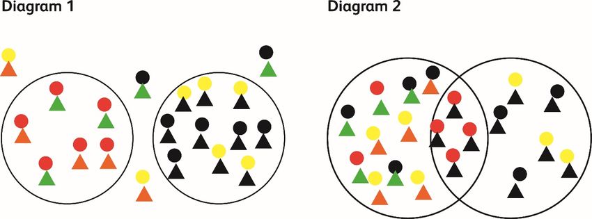
They concluded that the case had been affected by ‘tunnel vision’ (in other words, seeking confirmatory
evidence by initially focusing only on deaths that could involve Lucia de Berk, and not sufficiently
considering alternative scenarios), and cast doubt on the evidence of poisoning of one child, suggesting
that test results had been misinterpreted.

As a result of the review, the case was reopened, with further investigation and a retrial. It was
subsequently shown that both alleged cases of poisoning were not supported, and de Berk was not on
the premises for two of the alleged murders. Apparently, the overall number of deaths at that particular
medical unit was also higher before she started working there. In April 2010, the appeals court in Arnhem
ruled that there was no evidence that Lucia de Berk had committed a crime in any of the 10 cases, and
she was acquitted.

   Three plane crashes happened in an eight-day period in July 2014. Do you think this is suspicious?

   Unpicking whether a set of events is a coincidence or not is not straightforward. We can start by
   considering the probability of the set of events occurring naturally (i.e. coincidentally), and then
   consider the probabilities of other explanations.

   For the plane crashes, David Spiegelhalter, Professor for the Public Understanding of Risk at the
   University of Cambridge, has calculated that the chance of at least three crashes in an eight-day
   window is very small - around 1 in 1000 (Spiegelhalter 2014). But the right question to ask is
   whether such a 'cluster' is surprising over a longer period of time. He found that the probability of
   such a cluster of plane crashes within a 10-year period was about 60 per cent – i.e. more likely
   than not. It is not sufficient simply to identify this cluster to say that it is a suspicious pattern,
   rather than simply a chance event.

A 60 Second Science podcast ‘Brain Seeks Patterns where None Exist’, in Scientific American, in 2008,
shows that people tend to see non-existent patterns. However, this ‘cognitive bias’ seems to be reduced if
you are relaxed.

   Kim Rossmo wrote in The Police Chief that: “Efforts to solve a crime by ‘working backwards’ (from
   the suspect to the crime, rather than from the crime to the suspect) are susceptible to errors of
   coincidence. These types of errors are often seen in the ‘solutions’ to such famous cases as Jack
   the Ripper.” The Lucia de Berk example also shows our tendency to link things together and create
   causal stories, as well as the need to carefully question when others might be doing the same.

   It’s also important to consider the difference between the probability of a specific coincidence
   occurring, as opposed to the probability of any coincidence occurring within a group of events.

©2017 – The Council of the Inns of Court (COIC) and the Royal Statistical Society (RSS)                     12
The probability of two people in a room of 30 sharing a birthday is approximately 0.71 - i.e. just over a 7
in 10 chance of it happening. In other words, it is more likely to happen than not.

If you are one of the 30 people in the room, the probability of any of the other 29 having the same
birthday as you is approximately 0.08. That’s less than one in ten chance of it happening. 2 In the first
case, we are calculating the probability of a coincidence of the type of ‘one person and another person
share a birthday’, in a group where there are many possible birthday pairings. In the second case, we are
looking for a specific case of a pair where one of the pair is you.

    A statistician can provide information to help the court understand the circumstances of the
    situation as it relates to the prosecution proposition and the defence proposition. It is not for the
    statistician to rule whether a set of events is a coincidence or not, guilt or not; that is for the court.

    References and further reading

    Richard D Gill, Piet Groeneboom and Peter de Jong, ‘Elementary Statistics on Trial (the case of Lucia de Berk)’
    (Richard D Gill, 2010)  accessed 5 October 2017
    Ronald Meester, Marieke Collins, Richard Gill, Michiel van Lambalgen, “On the (ab)use of statistics in the legal
    case against the nurse Lucia de B.” (2006) 5 Law, Probability and Risk 233
    Openbaar Ministeriem, ‘Rapport Commissie evaluatie afgesloten strafzaken inzake mevrouw de B.’, 29 October
    2007.
    D. Kim Rossmo, ‘Failures in Criminal Investigation’ The Police Chief (October 2009) 54
    Scientific American, ‘Brain Seeks Patterns where None Exist’ (Scientific American, 3 October 2008)
     accessed 5
    October 2017
    David Spiegelhalter, ‘Another tragic cluster - but how surprised should we be?’ (Understanding Uncertainty, 25
    July 2014)  accessed
    5 October 2017

1.3 Independence
    If the occurrence of an event has no effect on the probability of another event then the two
    events are said to be independent. There is no relationship between them. Where the outcomes
    are independent you can multiply the associated probabilities together to get the probability of
    the two outcomes occurring. But if the outcomes are related or dependent you cannot do so. Note
    that the relationship may not be obvious. Many pairs of outcomes that look independent are not
    (see 2.1 Basic probability for a further explanation).

2
  For a full explanation of the mathematics of this, see https://www.mathsisfun.com/data/probability-shared-birthday.html for an
illustrated example

©2017 – The Council of the Inns of Court (COIC) and the Royal Statistical Society (RSS)                                      13
A variable is a statistical term that refers to a quantity that could in principle vary or differ – for example, height of one person over different times of the day, or height of different people across a population. An event is an outcome that can either happen or not. Variables and events can both have a quality called independence. In the case of the theft of the purse in Los Angeles described in 1.1 Misunderstandings of probability, the expert witness multiplied individual probabilities together to get 1 in 12,000,000 as the probability of any couple at random having all of six characteristics, such as “girl with blond hair” and “man with moustache”. Some of the stated identifiers are related and so cannot be multiplied together. In overturning the conviction, the Californian Supreme Court pointed out that since many black men have both beards and moustaches (including the defendant), there was “no basis” for multiplying the probability values for black men with beards and men with moustaches as these are not independent (People v Collins, 1968). Sally Clark, a British solicitor, was convicted in 1999 of murdering two of her sons. One died shortly after birth in 1996, and another in 1998. The prosecution case included flawed statistical evidence given by an expert witness paediatrician who asserted that the chance of two children from a professional non- smoking family dying from Sudden Infant Death Syndrome (SIDS) was 1 in 73 million. The figure of 1 in 73 million relied on a report which concluded that the possibility of a single SIDS in a similar family to Clark’s was 1 in 8,453. To reflect the two deaths, this probability was then squared to reach 1 in 73 million. The witness had presumed that each death was independent of the other and therefore multiplied the associated fractional probabilities of each death. The assumption of independence is not correct since there was evidence available that other factors, genetic or environmental, could have affected both children. A second appeal in 2003 overturned the conviction when it was found that there had been a failure to disclose medical reports suggesting that the second son had died of natural causes. After her release, Sally Clark developed severe psychiatric problems and died from alcohol poisoning in 2007. As the RSS said about the case of Sally Clark: “The calculation leading to 1 in 73 million is invalid. It would only be valid if SIDS cases arose independently within families, an assumption that would need to be justified empirically.” (Green 2002). In general, “independence must be demonstrated and verified before the product rule for independent events can safely be applied” (Aitken et al. 2010). The Law Commission (2011) considered the Sally Clark case when recommending reforms for managing expert witnesses and said that if its reforms had been in place: “the trial judge would have ruled on the scope of the paediatrician’s competence to give expert evidence and would ©2017 – The Council of the Inns of Court (COIC) and the Royal Statistical Society (RSS) 14
have monitored his evidence to ensure that he did not drift into other areas.” It added: “The
   paediatrician would not have been asked questions in the witness box on matters beyond his
   competence; and if he was inadvertently asked such a question … the judge would have
   intervened to prevent an impermissible opinion being given”.

   Additionally, if the Commission’s reforms had been in place, the “defence or court would
   presumably have raised the matter as a preliminary issue in the pre-trial proceedings and the
   judge would no doubt have directed that the parties and their experts attend a pre-trial hearing to
   assess the reliability of the figure… The reliability of the hypothesis (or assumption) … would then
   have been examined against our proposed statutory test, examples and factors. The expert would
   have been required to demonstrate the evidentiary reliability (the scientific validity) of his
   hypothesis and the chain of reasoning leading to his opinion, with reference to properly conducted
   scientific research and an explanation of the limitations in the research findings and the margins
   of uncertainty ...”

   The Law Commission believed that, had this approach been followed, it “would probably have
   provided a distinct basis upon which to quash C’s [Clark’s] convictions” and that if a competent
   statistician had provided a more “reliable figure as to the probability of two SIDS deaths in one
   family … under our recommendations that expert would have been expected to try to formulate a
   counterbalancing probability reflecting the defence case.”

   Note that the Law Commission’s reforms have not been implemented in the form proposed by
   the Commission. See Section 4: Current and future issues for discussion.

   References

   Colin Aitken, Paul Roberts, Graham Jackson, Fundamentals of probability and statistical evidence in criminal
   proceedings (Royal Statistical Society 2010)
   Peter Green, ‘Letter from the President to the Lord Chancellor regarding the use of statistical evidence in court
   cases’ (Royal Statistical Society, 23 January 2002)  accessed 5 October 2017
   Law Commission, Expert Evidence in Criminal Proceedings in England and Wales (Law Com No. 325, 2011)
   People v. Collins, 68 Cal.2d 319. [Crim. No. 11176. In Bank. Mar. 11, 1968.]
   R v Clark [2000] EWCA Crim 54; [2003] EWCA Crim 1020.

©2017 – The Council of the Inns of Court (COIC) and the Royal Statistical Society (RSS)                           15
1.4 Absolute and relative risk
   Risk has different meanings or interpretations, depending on the legal, professional or social
   context. In finance, for example, risk may be shorthand for potential financial loss, or financial
   volatility. In everyday language, risk usually refers to the possibility of an outcome that is
   negative. In statistics, risk usually refers to the probability that an event will occur. This may be a
   good or a bad event. In epidemiology, risk usually denotes a measure of disease frequency (see
   definition of relative risk below).

   In this guide, risk refers to the probability that an event will occur. In law, that event will
   constitute the harmful outcome that forms the basis of the legal claim. Two concepts of risk that
   often arise for consideration in tort litigation are relative risk and absolute risk, with the former
   being much more common.

   Relative risk (RR) describes the proportional increase in the probability of an effect of an event
   occurring to a group, as measured from a baseline of a comparison group that has not
   experienced the event. The important point to take from this definition is that a statistical result
   can only properly be expressed in the form of a relative risk if it derives from a study in which one
   group with the relevant characteristic is compared with a control group over a specified period of
   time. The characteristic being studied may relate, for example, to the onset of a particular disease
   or to exposure to a harmful agent such as asbestos. That the ‘RR’ label can only attach to results
   stemming from rigorously implemented studies of this nature is a point that cannot be stressed
   enough. It should be borne in mind when looking at recent toxic tort cases. Questions to consider
   include: what is the source of the statistical figures being relied upon as indicators of factual
   causation? Is there a scientific basis for them? Are the studies relied upon relevant to the claimant
   in terms of age, gender and lifestyle? What generalizations have been made and are they
   tenable?

   Absolute risk (AR) describes the overall risk to a population (or any other category) of an event –
   the probability of the event happening to any one member of the population. As such, it is not a
   term of art in the same way as relative risk. Indeed, it will often be the case that this statistic will
   have been extrapolated from an epidemiologic RR study. When assessing the relevance and
   reliability of such a statistic as regards the legal issue at stake, it will be of vital importance to look
   to the source of the information on which the AR calculation has been based. For instance, if the
   study in question was designed to measure the prevalence of lung cancer in women smokers aged
   between 25 to 40 years, it will not be relevant to a claimant who is male and/or a non-smoker. The
   smaller the study, the harder it will be to draw generalisations from it. In terms of assessing the
   scientific reliability of the data, obvious factors to look at will include the size of the P value (see

©2017 – The Council of the Inns of Court (COIC) and the Royal Statistical Society (RSS)                    16
2.3 The scientific method) or confidence interval (see 2.2 Inferential statistics and probability),
   and the measures taken to guard against biases (for example, bias in the selection of cases for a
   study) and confounders (see the ice cream and sunglasses example in 1.5 Correlation and
   causation below).

   Consider the following example. If you read: “People who use sunbeds are 20% more likely to
   develop malignant melanoma”, this relates to the relative risk of developing cancer (assuming it
   derives from a reliable epidemiologic study with the all-important control group). This percentage
   on its own does not tell us what the overall likelihood is of developing this kind of cancer ‒ in other
   words, the absolute risk.

   Cancer Research UK has usefully explored the importance of understanding these differences.
   Williams (2013) noted that The Guardian reported a 70% increase in thyroid cancer amongst
   women after the Fukushima nuclear disaster in 2011. This is a relative risk. A 70% increase sounds
   alarming – but it does not tell us what proportion of the population would be affected. The Wall
   Street Journal reported that the absolute risk of this cancer was low (about 0.77% - that’s
   seventy-seven out of ten thousand people). A 70% increase in risk would take it to an incidence of
   1.29 per cent in the population. That increase in absolute risk is 0.52 percentage points. For a
   population of 10,000, an extra 52 people would be affected. Expressing these changes in absolute
   risk allows for fair comparisons between different activities. For example, if another (fictitious)
   cancer had increased by 35% after Fukushima, but had an existing absolute risk of 2%, then the
   second cancer would have an extra 70 cases in 10,000 (from 200 per 10,000 to 270 per 10,000).
   In this example, although the change in relative risk was smaller (35% rather than 70%), the
   overall effect on the population was larger (an extra 70 cancer cases compared with an extra 52
   cancer cases).

   The important point to take away from the above example is that the same raw data can be used
   to make a number of different statistical calculations and so, when you are looking at expert
   evidence involving statistical results, you will need to know what calculations have been made and
   be able to explain the specific nature of the risk being presented. You will need to be able to
   determine at the case management stage the relevance and significance, or lack thereof, of the
   calculations to the specific legal issues you are dealing with.

   References and further reading
   Choudhury v South Central Ambulance Service NHS [2015] EWHC 1311 (QB) (an example of incorrect use of
   the technical term ‘relative risk’.)
   Sarah Williams, ‘Absolute versus relative risk – making sense of media stories’, (Cancer Research UK, 15 March
   2013)  accessed 5 October 2017

©2017 – The Council of the Inns of Court (COIC) and the Royal Statistical Society (RSS)                        17
1.5 Correlation and causation
    Complex phenomena with multiple potential relationships and impacts are sometimes explored
    by looking at correlations between variables rather than conducting an experiment (see 2.3 The
    scientific method). This ‘observational’ method is used quite often in medicine to observe or
    indicate a link between various variables. It does not ‘prove’ causation but can be highly
    indicative of a relationship and lead to further research to determine causal mechanisms.

In 1965, an expert witness told a US Senate committee hearing that even though smoking might be
correlated with lung cancer, any causal relationship was unproven as well as implausible. This followed
the 1964 Report on Smoking and Health of the Surgeon General, which found correlations between
smoking and chronic bronchitis, emphysema, and coronary heart disease. 3

    This example might at first glance be seen to illustrate the mantra that – ‘Correlation does not
    equal causation’. However, it is important to realise that many medical studies are, in fact, based
    on correlations between variables since the underlying causal mechanisms are not yet fully
    understood. These are called epidemiological studies.

The expert witness at the US Senate committee hearing on smoking, referred to above, was Darrel Huff.
An esteemed populariser of statistics (see Further resources), he was not a qualified statistician. His
testimony, and an unpublished book on the case for smoking, made statistical mistakes and did not look
at the whole view (Reinhart 2014).

Correlations can be measured by specific statistics which calculate the likely extent of the ‘relationship’
between variables. An example is the Pearson Correlation Coefficient which calculates a number
between -1 and +1 to describe the strength and form of the linear correlation. For example, +0.9
indicates a high positive correlation – as one value goes up, so does the other. If the result is 0, there is
likely to be no linear relationship (although there may be another kind of relationship). If the coefficient
is -0.5 there is a low negative correlation – as one value increases, the other decreases.

The Pearson Correlation Coefficient works only for linear relationships. There might be a curved pattern
or relationship which would not be picked up. The charts overleaf illustrate this:

3
 See U.S. National Library of Medicine, ‘The Reports of the Surgeon General: The 1964 Report on Smoking and Health’ (Profiles in
Science, undated)  accessed 5 October 2017

©2017 – The Council of the Inns of Court (COIC) and the Royal Statistical Society (RSS)                                     18
These data have a Pearson Correlation These data have a Pearson Correlation
Coefficient of 0.8 Coefficient of 0.2
100 100
80 80
60 60
40 40
20 20
0 0
0 20 40 60 80 100 0 20 40 60 80 100
These data have a Pearson Correlation These data have a Pearson Correlation
Coefficient of -0.5 Coefficient of 0
100 100
80 80
60 60
40 40
20 20
0 0
0 20 40 60 80 100 0 20 40 60 80 100
You have to be careful when considering correlation. Even if two variables seem to have a strong
relationship, one variable may not in fact be the cause of another. This is what is called a
‘spurious’ correlation.
An amusing website by Tyler Vigen provides a range of examples, one of which, for example, shows that
per capita US cheese consumption correlates with death from becoming tangled in bed sheets in the
USA. The correlation coefficient is 0.95 which is quite high. Any such observed link might just result from
two independent trends that are going in similar directions.
An observed correlation might also be caused by another or confounding variable that affects
both. Consider this simple example of a plot of values of weekly ice cream sales against weekly
values of sunglasses sales.
©2017 – The Council of the Inns of Court (COIC) and the Royal Statistical Society (RSS) 19Weekly sales of sunglasses and ice-cream at
Fictum Beach Hut
600
500
Weekly sales in GBP (£)
400
300
200
100
0
0 2 4 6 8 10 12 14
Week number (current financial year)
Total income from sunglasses per week (£) Total income from icecream per week (£)
Even if the sale of sunglasses and sales of ice cream seem to vary together, it is obvious that one
does not cause the other. Rather, the weather causes changes in the sales of both.
Ice cream sales
Weather
Sunglasses sales
You cannot just dismiss correlations as not indicating a cause or direct link between two variables.
It may not yet have been proven. A well-conducted statistical experiment can you give very
convincing evidence of causation. Subsequent studies may provide further evidence for the
hypothesis. In the case of smoking, for example, the links between smoking and lung cancer have
been supported by subsequent experimental scientific studies as well as observational studies.
You may need to probe further to see if there is evidence to explain the correlation – is it
accidental, or an as yet unproven but strongly suggestive relationship, or is it just caused by
something else?
©2017 – The Council of the Inns of Court (COIC) and the Royal Statistical Society (RSS) 20Epidemiology and tort litigation
Epidemiology is best understood as a public health science that looks at the causes and
determinants of diseases in human populations. It is primarily used to help develop health
strategies for general populations. A recent example of its application in a health policy context
are the bans on smoking in public spaces across the UK owing to the various risks of harm
associated with second-hand smoke. There is also a growing trend of using epidemiologic research
in tort litigation where the actionable damage is a complex disease (i.e. a disease about which
there are significant gaps in medical knowledge). The legal claims involved tend to fall into three
categories: (1) toxic torts (where the disease allegedly results from exposure to a toxic substance);
(2) medical negligence claims, e.g. where a doctor is sued for failing to diagnose the relevant
disease in a timely fashion; and (3) pharmaceutical products liability under the Consumer
Protection Act 1987. In the vast majority of these claims, the epidemiological evidence is used at
the factual causation stage of the legal enquiry (although note that in product liability claims, it is
also used to determine the whether the product is defective – see XYZ v Schering Health Care
[2002] EWHC 1420 (QB)).
The science of epidemiology is expressly concerned with probabilities. For this reason, it will be
less often of use in criminal cases given the high standard of proof required, though relevant
epidemiology might still properly provide support for the prosecution in, say, a medical
manslaughter case if there is other evidence of guilt. 4 In civil law, the balance of probabilities
standard allows for more uncertainty than the beyond reasonable doubt standard of criminal law
– the evidence presented need only persuade the court that it is more likely than not that the
relevant legal issue (for present purposes, it is factual causation) has been established.
Using epidemiology to decide questions of causation is controversial. 5 The court in a toxic tort
case is applying a statistical model derived from the epidemiology to the facts of a single case. In
doing so the court is using epidemiological data for a very different purpose from that of the
researchers. See further in Section 4: Current and future issues.
Epidemiologists employ a variety of bespoke methodologies to collect and interpret data and the
calculation of incidence and prevalence rates count among the most basic of these. Methods
include ecological studies (comparing groups of people separated by time, location or
characteristic), longitudinal or cohort studies (tracking groups of people over time), case-control
4
And it might be deployed in such a case by the defendant on whom no burden of proof lies.
5
Reservations about its use in tort litigation were recorded by members of the Supreme Court in Sienkiewicz v Greif (UK) Ltd [2011]
2 AC 229 though arguably some of the concerns are based on a misunderstanding of the methodologies used by epidemiologists
to derive conclusions from datasets: see Claire McIvor, ‘Debunking some judicial myths about epidemiology and its relevance to
UK tort law’ [2013] Medical Law Review 553
©2017 – The Council of the Inns of Court (COIC) and the Royal Statistical Society (RSS) 21studies (examining the life histories of people with cases of disease), cross-sectional studies,
performing experiments including randomised controlled trials, and analysing data from
screening and outbreaks of diseases (see Coggon et al. for a description). The type of study can
affect its accuracy and reliability. A longitudinal study can be prospective whilst a case-control
study is retrospective. Retrospective studies are more prone to confounding and bias.
If a statistically significant relationship is found between an agent and a health outcome, one of
the methods subsequently used to determine whether that relationship is indicative of a
biologically causal relationship is the Bradford Hill guidelines.
Bradford Hill guidelines
Sir Austin Bradford Hill, in his President's Address in 1965 to the Section of Occupational Medicine
of the Royal Society of Medicine, gave a list of aspects of association which could be useful in
assessing whether an association between two variables should be interpreted as a causal
relationship. These have become known in epidemiology as the Bradford Hill guidelines and are
used in debates such as whether mobile telephone use can cause brain tumours.
The aspects of association, or guidelines, are:
• Strength: the strength of the association, for example, the death rate from lung cancer in
smokers is ten times the rate in non-smokers, and heavy smokers have a lung cancer death
rate twenty times that of non-smokers.
• Consistency: if an association is repeatedly observed by different people, in different places,
circumstances and times, it is more reasonable to conclude that the association is not due to
error, or imprecise definition, or a false positive statistical result.
• Specificity: consideration should be given to whether particular diseases only occur among
workers in particular occupations, or if there are particular causes of death. This is a
supporting feature in some cases, but in other cases one agent might give rise to a range of
reasons for death.
• Temporality: this requires causal factors to be present before the disease.
• Dose-response curve, or biological gradient: if the frequency of a disease increases as
consumption or exposure to a factor increases, this supports a causal association. Increasing
levels of smoking, or of exposure to silicon dust associated with increased frequency of lung
disease supports the hypothesis that smoking or silicon dust causes lung disease.
©2017 – The Council of the Inns of Court (COIC) and the Royal Statistical Society (RSS) 22• Plausibility: if the causation suspected is biologically plausible. However, the association
observed may be one new to science or medicine, and still be valid.
• Coherence: a cause and effect interpretation should not seriously conflict with generally
known facts of the development and biology of the disease.
• Experiment: sometimes evidence from laboratory or field experiments might be available.
• Analogy: if there is strong evidence of a causal relationship between a factor and an effect,
it could be fair to accept “slighter but similar evidence” between a similar factor and a
similar effect.
Hill himself was keen to stress that “none of my nine viewpoints can bring indisputable evidence
for or against the cause-and-effect hypothesis and none can be required as a sine qua non” (Hill
1965). Conversely, if none of the guidelines is met, one cannot conclude that there is not a causal
association. The conclusion is that there might be a direct causal explanation, or an indirect
explanation, or even that the association arose from some aspects of data collection or analysis.
Epidemiologists may also consider competing explanations, such as an unmeasured confounding
factor, an alternative factor which has an association of similar strength to the putative causal
factor. For example, high alcohol consumption is associated with lung cancer. As people who drink
often also smoke, before no smoking areas were common, pubs were often full of smoke. One
should consider if the effects of drinking and smoking can be distinguished.
References and further information
D Coggon, Geoffrey Rose, DJP Barker, Epidemiology for the uninitiated, (Fourth edition, BMJ Books). Available
online at
N Duan, RL Kravitz, CH Schmid. ‘Single-patient (n-of-1) trials: a pragmatic clinical decision methodology for
patient-centered comparative effectiveness research’ (2013) 66(8 0) Supplement Journal of Clinical
Epidemiology 21 Author manuscript available at https://www.ncbi.nlm.nih.gov/pmc/articles/PMC3972259/
Austin Bradford Hill, ‘The Environment and Disease: Association or Causation?’ [1965] Proceedings of the Royal
Society of Medicine 295
Claire McIvor, ‘Debunking some judicial myths about epidemiology and its relevance to UK tort law’ [2013]
Medical Law Review 553
Rod Pierce, ‘Correlation’ (Math Is Fun, 27 Jan 2017) accessed 6
October 2017
Alex Reinhart, ‘Huff and puff’ (2014) 11(4) Significance 28
Sienkiewicz v Greif (UK) Ltd [2011] UKSC 10; [2011] 2 AC 229
Tyler Vigen, 'Spurious Correlations' (Spurious Correlations, undated) accessed 12 October 2017
For more on smoking, correlation and causation, see the Financial Times article Cigarettes, damn cigarettes and
statistics by Tim Harford (10 April 2015), which shows how evidence of causality in relation to the impacts of
cigarette smoke on health was built over time from correlation, through the timing of effects and relative dose
and impact levels.
©2017 – The Council of the Inns of Court (COIC) and the Royal Statistical Society (RSS) 231.6 False positives and false negatives Tests are often used in forensic science and medicine to determine whether a person has a particular characteristic, such as a blood type or an illness. Forensic tests may be carried out, for example, on products such as food, or other consumer goods, or construction materials. Like any measurement process, they are subject to error which can arise from many sources − bias, inappropriate calibration, human error mixing samples, and random variation. It is important to know what this error might be, since a test, say for evidence, might incorrectly identify a match when there isn’t one, or alternatively not identify a match when there is one. In relation to medicine, a test for cancer might not show it is there when it is or, alternatively, might identify cancer when it is not there. In 2003, a student was arrested in Philadelphia airport. Her luggage contained three condoms filled with a white powder which a field test indicated was cocaine. The student argued that these were flour and she used them as stress relief toys for exams. She spent the next three weeks in jail on drug charges until an attorney encouraged the state prosecutor to arrange laboratory testing. The tests confirmed that the powder was flour. Ultimately, she was awarded $180,000 compensation by Philadelphia. She had been arrested and held in jail on a ‘false positive’ result. With scientific or medical tests, a false positive result is one in which the test gives a positive result indicating the presence of the substance or disease for which the test was conducted when, in reality, that substance or disease is not present. A false negative result is one in which the test gives a negative result indicating the absence of the substance or disease for which the test was conducted when in fact the substance or disease is present. The rates of false positives and false negatives (a measure of the reliability of the testing procedure) can be used to assign probabilities of observing false positives and false negatives as if the tests were applied across a population. Even very reliable tests (those with a low false positive rate) could lead to declared matches being false for many test results. This example illustrates this. Imagine 1000 people. 10 have a disease (a prevalence of 1%). 990 don’t have the disease. All 1000 people are tested for that disease at the same time. The test used is known to have a false positive rate of 10% and a false negative rate of 20%. A false negative rate of 20% means that of those 10 with the disease, only 8 are correctly identified as having the disease. The false positive rate of 10% means that this test will identify wrongly 10% of those 990 who do not have the disease as having the disease. At the end of the test across all 1000 people, we are therefore left with 107 people testing positive (8 + 99), but only 8 need treatment (that’s about 7% of ©2017 – The Council of the Inns of Court (COIC) and the Royal Statistical Society (RSS) 24
You can also read