Jet reconstruction and performance using particle flow with the ATLAS Detector - arXiv
←
→
Page content transcription
If your browser does not render page correctly, please read the page content below
EUROPEAN ORGANISATION FOR NUCLEAR RESEARCH (CERN)

                                          Eur. Phys. J. C 77 (2017) 466                                                                   CERN-EP-2017-024
                                          DOI: 10.1140/epjc/s10052-017-5031-2                                                               15th August 2017
arXiv:1703.10485v2 [hep-ex] 14 Aug 2017

                                           Jet reconstruction and performance using particle
                                                     flow with the ATLAS Detector

                                                                                 The ATLAS Collaboration

                                                 This paper describes the implementation and performance of a particle flow algorithm applied
                                                 to 20.2 fb−1 of ATLAS data from 8 TeV proton–proton collisions in Run 1 of the LHC. The
                                                 algorithm removes calorimeter energy deposits due to charged hadrons from consideration
                                                 during jet reconstruction, instead using measurements of their momenta from the inner
                                                 tracker. This improves the accuracy of the charged-hadron measurement, while retaining
                                                 the calorimeter measurements of neutral-particle energies. The paper places emphasis on
                                                 how this is achieved, while minimising double-counting of charged-hadron signals between
                                                 the inner tracker and calorimeter. The performance of particle flow jets, formed from the
                                                 ensemble of signals from the calorimeter and the inner tracker, is compared to that of
                                                 jets reconstructed from calorimeter energy deposits alone, demonstrating improvements in
                                                 resolution and pile-up stability.

                                          © 2017 CERN for the benefit of the ATLAS Collaboration.
                                          Reproduction of this article or parts of it is allowed as specified in the CC-BY-4.0 license.
Contents
1   Introduction                                                                                     3

2   ATLAS detector                                                                                   5

3   Simulated event samples                                                                          7
    3.1 Detector simulation and pile-up modelling                                                    7
    3.2 Truth calorimeter energy and tracking information                                            8

4   Data sample                                                                                      8

5   Topological clusters                                                                             9

6   Particle flow algorithm                                                                          9
    6.1 Containment of showers within a single topo-cluster                                         10
    6.2 Track selection                                                                             13
    6.3 Matching tracks to topo-clusters                                                            15
    6.4 Evaluation of the expected deposited particle energy through hEref
                                                                       clus /ptrk i determination
                                                                              ref                   18
    6.5 Recovering split showers                                                                    20
    6.6 Cell-by-cell subtraction                                                                    22
    6.7 Remnant removal                                                                             22

7   Performance of the subtraction algorithm at truth level                                         22
    7.1 Track–cluster matching performance                                                          23
    7.2 Split-shower recovery performance                                                           25
    7.3 Accuracy of cell subtraction                                                                25
    7.4 Visualising the subtraction                                                                 27

8   Jet reconstruction and calibration                                                              28
    8.1 Overview of particle flow jet calibration                                                   30
    8.2 Area-based pile-up correction                                                               30
    8.3 Monte Carlo numerical inversion                                                             30
    8.4 Global sequential correction                                                                32
    8.5 In situ validation of JES                                                                   32

9   Resolution of jets in Monte Carlo simulation                                                    33
    9.1 Transverse momentum resolution                                                              33
    9.2 Angular resolution of jets                                                                  34

10 Effect of pile-up on the jet resolution and rejection of pile-up jets                            35
   10.1 Pile-up jet rate                                                                            35
   10.2 Pile-up effects on jet energy resolution                                                    38

11 Comparison of data and Monte Carlo simulation                                                    39
   11.1 Individual jet properties                                                                   40
   11.2 Event-level observables                                                                     40

12 Conclusions                                                                                      44

                                                    2
1 Introduction
Jets are a key element in many analyses of the data collected by the experiments at the Large Hadron
Collider (LHC) [1]. The jet calibration procedure should correctly determine the jet energy scale and
additionally the best possible energy and angular resolution should be achieved. Good jet reconstruction
and calibration facilitates the identification of known resonances that decay to hadronic jets, as well as the
search for new particles. A complication, at the high luminosities encountered by the ATLAS detector [2],
is that multiple interactions can contribute to the detector signals associated with a single bunch-crossing
(pile-up). These interactions, which are mostly soft, have to be separated from the hard interaction that is
of interest.
Pile-up contributes to the detector signals from the collision environment, and is especially important
for higher-intensity operations of the LHC. One contribution arises from particle emissions produced
by the additional proton–proton (pp) collisions occurring in the same bunch crossing as the hard-scatter
interaction (in-time pile-up). Further pile-up influences on the signal are from signal remnants in the
ATLAS calorimeters from the energy deposits in other bunch crossings (out-of-time pile-up).
In Run 1 of the LHC, the ATLAS experiment used either solely the calorimeter or solely the tracker to
reconstruct hadronic jets and soft particle activity. The vast majority of analyses utilised jets that were
built from topological clusters of calorimeter cells (topo-clusters) [3]. These jets were then calibrated to
the particle level using a jet energy scale (JES) correction factor [4–7]. For the final Run 1 jet calibration,
this correction factor also took into account the tracks associated with the jet, as this was found to greatly
improve the jet resolution [4]. ‘Particle flow’ introduces an alternative approach, in which measurements
from both the tracker and the calorimeter are combined to form the signals, which ideally represent
individual particles. The energy deposited in the calorimeter by all the charged particles is removed. Jet
reconstruction is then performed on an ensemble of ‘particle flow objects’ consisting of the remaining
calorimeter energy and tracks which are matched to the hard interaction.
The chief advantages of integrating tracking and calorimetric information into one hadronic reconstruction
step are as follows:
• The design of the ATLAS detector [8] specifies a calorimeter energy resolution for single charged
pions in the centre of the detector of
σ(E) 50 % 1%
= √ ⊕ 3.4 % ⊕ , (1)
E E E
while the design inverse transverse momentum resolution for the tracker is
1
σ · pT = 0.036 % · pT ⊕ 1.3 % , (2)
pT
where energies and transverse momenta are measured in GeV. Thus for low-energy charged particles,
the momentum resolution of the tracker is significantly better than the energy resolution of the
calorimeter. Furthermore, the acceptance of the detector is extended to softer particles, as tracks are
reconstructed for charged particles with a minimum transverse momentum pT > 400 MeV, whose
energy deposits often do not pass the noise thresholds required to seed topo-clusters [9].
• The angular resolution of a single charged particle, reconstructed using the tracker is much better
than that of the calorimeter.
3• Low-pT charged particles originating within a hadronic jet are swept out of the jet cone by the
magnetic field by the time they reach the calorimeter. By using the track’s azimuthal coordinate1 at
the perigee, these particles are clustered into the jet.
• When a track is reconstructed, one can ascertain whether it is associated with a vertex, and if so the
vertex from which it originates. Therefore, in the presence of multiple in-time pile-up interactions,
the effect of additional particles on the hard-scatter interaction signal can be mitigated by rejecting
signals originating from pile-up vertices.2
The capabilities of the tracker in reconstructing charged particles are complemented by the calorimeter’s
ability to reconstruct both the charged and neutral particles. At high energies, the calorimeter’s energy
resolution is superior to the tracker’s momentum resolution. Thus a combination of the two subsystems
is preferred for optimal event reconstruction. Outside the geometrical acceptance of the tracker, only the
calorimeter information is available. Hence, in the forward region the topo-clusters alone are used as
inputs to the particle flow jet reconstruction.
However, particle flow introduces a complication. For any particle whose track measurement ought to be
used, it is necessary to correctly identify its signal in the calorimeter, to avoid double-counting its energy
in the reconstruction. In the particle flow algorithm described herein, a Boolean decision is made as to
whether to use the tracker or calorimeter measurement. If a particle’s track measurement is to be used,
the corresponding energy must be subtracted from the calorimeter measurement. The ability to accurately
subtract all of a single particle’s energy, without removing any energy deposited by any other particle,
forms the key performance criterion upon which the algorithm is optimised.
Particle flow algorithms were pioneered in the ALEPH experiment at LEP [10]. They have also been
used in the H1 [11], ZEUS [12, 13] and DELPHI [14] experiments. Subsequently, they were used for
the reconstruction of hadronic τ-lepton decays in the CDF [15], D0 [16] and ATLAS [17] experiments.
In the CMS experiment at the LHC, large gains in the performance of the reconstruction of hadronic jets
and τ leptons have been seen from the use of particle flow algorithms [18–20]. Particle flow is a key
ingredient in the design of detectors for the planned International Linear Collider [21] and the proposed
calorimeters are being optimised for its use [22]. While the ATLAS calorimeter already measures jet
energies precisely [6], it is desirable to explore the extent to which particle flow is able to further improve
the ATLAS hadronic-jet reconstruction, in particular in the presence of pile-up interactions.
This paper is organised as follows. A description of the detector is given in Section 2, the Monte Carlo
(MC) simulated event samples and the dataset used are described in Sections 3 and 4, while Section 5
outlines the relevant properties of topo-clusters. The particle flow algorithm is described in Section 6.
Section 7 details the algorithm’s performance in energy subtraction at the level of individual particles in
a variety of cases, starting from a single pion through to dijet events. The building and calibration of
reconstructed jets is covered in Section 8. The improvement in jet energy and angular resolution is shown
in Section 9 and the sensitivity to pile-up is detailed in Section 10. A comparison between data and MC
simulation is shown in Section 11 before the conclusions are presented in Section 12.
1 ATLAS uses a right-handed coordinate system with its origin at the nominal interaction point (IP) in the centre of the detector
and the z-axis along the beam direction. The x-axis points from the IP to the centre of the LHC ring, and the y-axis points
upward. Cylindrical coordinates (r, φ) are used in the transverse plane, φ being the azimuthal angle around the z-axis.
The pseudorapidity
p is defined in terms of the polar angle θ as η = − ln tan(θ/2). Angular distance is measured in units of
∆R = (∆φ)2 + (∆η)2 .
2 The standard ATLAS reconstruction defines the hard-scatter primary vertex to be the primary vertex with the largest Í p2 of
T
the associated tracks. All other primary vertices are considered to be contributed by pile-up.
42 ATLAS detector
The ATLAS experiment features a multi-purpose detector designed to precisely measure jets, leptons and
photons produced in the pp collisions at the LHC. From the inside out, the detector consists of a tracking
system called the inner detector (ID), surrounded by electromagnetic (EM) sampling calorimeters. These
are in turn surrounded by hadronic sampling calorimeters and an air-core toroid muon spectrometer (MS).
A detailed description of the ATLAS detector can be found in Ref. [2].
The high-granularity silicon pixel detector covers the vertex region and typically provides three meas-
urements per track. It is followed by the silicon microstrip tracker which usually provides eight hits,
corresponding to four two-dimensional measurement points, per track. These silicon detectors are com-
plemented by the transition radiation tracker, which enables radially extended track reconstruction up
to |η| = 2.0. The ID is immersed in a 2 T axial magnetic field and can reconstruct tracks within the
pseudorapidity range |η| < 2.5. For tracks with transverse momentum pT < 100 GeV, the fractional
inverse momentum resolution σ(1/pT ) · pT measured using 2012 data, ranges from approximately 2 % to
12 % depending on pseudorapidity and pT [23].
The calorimeters provide hermetic azimuthal coverage in the range |η| < 4.9. The detailed structure
of the calorimeters within the tracker acceptance strongly influences the development of the shower
subtraction algorithm described in this paper. In the central barrel region of the detector, a high-
granularity liquid-argon (LAr) electromagnetic calorimeter with lead absorbers is surrounded by a hadronic
sampling calorimeter (Tile) with steel absorbers and active scintillator tiles. The same LAr technology
is used in the calorimeter endcaps, with fine granularity and lead absorbers for the EM endcap (EMEC),
while the hadronic endcap (HEC) utilises copper absorbers with reduced granularity. The solid angle
coverage is completed with forward copper/LAr and tungsten/LAr calorimeter modules (FCal) optimised
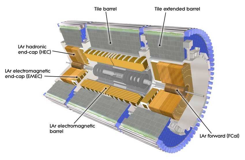
for electromagnetic and hadronic measurements respectively. Figure 1 shows the physical location of
the different calorimeters. To achieve a high spatial resolution, the calorimeter cells are arranged in
a projective geometry with fine segmentation in φ and η. Additionally, each of the calorimeters is
longitudinally segmented into multiple layers, capturing the shower development in depth. In the region
|η| < 1.8, a presampler detector is used to correct for the energy lost by electrons and photons upstream of
the calorimeter. The presampler consists of an active LAr layer of thickness 1.1 cm (0.5 cm) in the barrel
(endcap) region. The granularity of all the calorimeter layers within the tracker acceptance is given in
Table 1.
The EM calorimeter is over 22 radiation lengths in depth, ensuring that there is little leakage of EM
showers into the hadronic calorimeter. The total depth of the complete calorimeter is over 9 interaction
lengths in the barrel and over 10 interaction lengths in the endcap, such that good containment of hadronic
showers is obtained. Signals in the MS are used to correct the jet energy if the hadronic shower is not
completely contained. In both the EM and Tile calorimeters, most of the absorber material is in the second
layer. In the hadronic endcap, the material is more evenly spread between the layers.
The muon spectrometer surrounds the calorimeters and is based on three large air-core toroid super-
conducting magnets with eight coils each. The field integral of the toroids ranges from 2.0 to 6.0 T m
across most of the detector. It includes a system of precision tracking chambers and fast detectors for
triggering.
5EM LAr calorimeter
Barrel Endcap
Presampler 0.025 × π/32 |η| < 1.52 0.025 × π/32 1.5 < |η| < 1.8
PreSamplerB/E
1st layer 0.025/8 × π/32 |η| < 1.4 0.050 × π/32 1.375 < |η| < 1.425
EMB1/EME1 0.025 × π/128 1.4 < |η| < 1.475 0.025 × π/32 1.425 < |η| < 1.5
0.025/8 × π/32 1.5 < |η| < 1.8
0.025/6 × π/32 1.8 < |η| < 2.0
0.025/4 × π/32 2.0 < |η| < 2.4
0.025 × π/32 2.4 < |η| < 2.5
0.1 × π/32 2.5 < |η| < 3.2
2nd layer 0.025 × π/128 |η| < 1.4 0.050 × π/128 1.375 < |η| < 1.425
EMB2/EME2 0.075 × π/128 1.4 < |η| < 1.475 0.025 × π/128 1.425 < |η| < 2.5
0.1 × π/32 2.5 < |η| < 3.2
3rd layer 0.050 × π/128 |η| < 1.35 0.050 × π/128 1.5 < |η| < 2.5
EMB3/EME3
Tile calorimeter
Barrel Extended barrel
1st layer 0.1 × π/32 |η| < 1.0 0.1 × π/32 0.8 < |η| < 1.7
TileBar0/TileExt0
2nd layer 0.1 × π/32 |η| < 1.0 0.1 × π/32 0.8 < |η| < 1.7
TileBar1/TileExt1
3rd layer 0.2 × π/32 |η| < 1.0 0.2 × π/32 0.8 < |η| < 1.7
TileBar2/TileExt2
Hadronic LAr calorimeter
Endcap
1st layer 0.1 × π/32 1.5 < |η| < 2.5
HEC0 0.2 × π/16 2.5 < |η| < 3.2
2nd layer 0.1 × π/32 1.5 < |η| < 2.5
HEC1 0.2 × π/16 2.5 < |η| < 3.2
3rd layer 0.1 × π/32 1.5 < |η| < 2.5
HEC2 0.2 × π/16 2.5 < |η| < 3.2
4th layer 0.1 × π/32 1.5 < |η| < 2.5
HEC3 0.2 × π/16 2.5 < |η| < 3.2
Table 1: The granularity in ∆η × ∆φ of all the different ATLAS calorimeter layers relevant to the tracking coverage
of the inner detector.
6Figure 1: Cut-away view of the ATLAS calorimeter system.
3 Simulated event samples
A variety of MC samples are used in the optimisation and performance evaluation of the particle flow
algorithm. The simplest samples consist of a single charged pion generated with a uniform spectrum in
the logarithm of the generated pion energy and in the generated η. Dijet samples generated with Pythia 8
(v8.160) [24, 25], with parameter values set to the ATLAS AU2 tune [26] and the CT10 parton distribution
functions (PDF) set [27], form the main samples used to derive the jet energy scale and determine the jet
energy resolution in simulation. The dijet samples are generated with a series of jet pT thresholds applied
to the leading jet, reconstructed from all stable final-state particles excluding muons and neutrinos, using
the anti-k t algorithm [28] with radius parameter 0.6 using FastJet (v3.0.3) [29, 30].
For comparison with collision data, Z → µµ events are generated with Powheg-Box (r1556) [31] using
the CT10 PDF and are showered with Pythia 8, with the ATLAS AU2 tune. Additionally, top quark
pair production is simulated with MC@NLO (v4.03) [32, 33] using the CT10 PDF set, interfaced with
Herwig (v6.520) [34] for parton showering, and the underlying event is modelled by Jimmy (v4.31) [35].
The top quark samples are normalised using the cross-section calculated at next-to-next-to-leading order
(NNLO) in QCD including resummation of next-to-next-to-leading logarithmic soft gluon terms with
top++2.0 [36–43], assuming a top quark mass of 172.5 GeV. Single-top-quark production processes
contributing to the distributions shown are also simulated, but their contributions are negligible.
3.1 Detector simulation and pile-up modelling
All samples are simulated using Geant4 [44] within the ATLAS simulation framework [45] and are
reconstructed using the noise threshold criteria used in 2012 data-taking [3]. Single-pion samples are
simulated without pile-up, while dijet samples are simulated under three conditions: with no pile-up; with
pile-up conditions similar to those in the 2012 data; and with a mean number of interactions per bunch
7crossing hµi = 40, where µ follows a Poisson distribution. In 2012, the mean value of µ was 20.7 and the
actual number of interactions per bunch crossing ranged from around 10 to 35 depending on the luminosity.
The bunch spacing was 50 ns. When compared to data, the MC samples are reweighted to have the same
distribution of µ as present in the data. In all the samples simulated including pile-up, effects from both the
same bunch crossing and previous/subsequent crossings are simulated by overlaying additional generated
minimum-bias events on the hard-scatter event prior to reconstruction. The minimum-bias samples are
generated using Pythia 8 with the ATLAS AM2 tune [46] and the MSTW2009 PDF set [47], and are
simulated using the same software as the hard-scatter event.
3.2 Truth calorimeter energy and tracking information
For some samples the full Geant4 hit information [44] is retained for each calorimeter cell such that the
true amount of hadronic and electromagnetic energy deposited by each generated particle is known. Only
the measurable hadronic and electromagnetic energy deposits are counted, while the energy lost due to
nuclear capture and particles escaping from the detector is not included. For a given charged pion the sum
clus i .
of these hits in a given cluster i originating from this particle is denoted by Etrue, π
Reconstructed topo-cluster energy is assigned to a given truth particle according to the proportion of
Geant4 hits supplied to that topo-cluster by that particle. Using the Geant4 hit information in the inner
detector a track is matched to a generated particle based on the fraction of hits on the track which originate
from that particle [48].
4 Data sample
Data acquired during the period from March to December 2012 with the LHC operating at a pp centre-of-
mass energy of 8 TeV are used to evaluate the level of agreement between data and Monte Carlo simulation
of different outputs of the algorithm. Two samples with a looser preselection of events are reconstructed
using the particle flow algorithm. A tighter selection is then used to evaluate its performance.
First, a Z → µµ enhanced sample is extracted from the 2012 dataset by selecting events containing two
reconstructed muons [49], each with pT > 25 GeV and |η| < 2.4, where the invariant mass of the dimuon
pair is greater than 55 GeV, and the pT of the dimuon pair is greater than 30 GeV.
Similarly, a sample enhanced in t t¯ → bb̄q q̄µν events is obtained from events with an isolated muon and
at least one hadronic jet which is required to be identified as a jet containing b-hadrons (b-jet). Events
are selected that pass single-muon triggers and include one reconstructed muon satisfying pT > 25 GeV,
|η| < 2.4, for which the sum of additional track momenta in a cone of size ∆R = 0.2 around the muon
track is less than 1.8 GeV. Additionally, a reconstructed calorimeter jet is required to be present with
pT > 30 GeV, |η| < 2.5, and pass the 70 % working point of the MV1 b-tagging algorithm [50].
For both datasets, all ATLAS subdetectors are required to be operational with good data quality. Each
dataset corresponds to an integrated luminosity of 20.2 fb−1 . To remove events suffering from signific-
ant electronic noise issues, cosmic rays or beam background, the analysis excludes events that contain
calorimeter jets with pT > 20 GeV which fail to satisfy the ‘looser’ ATLAS jet quality criteria [51, 52].
85 Topological clusters
The lateral and longitudinal segmentation of the calorimeters permits three-dimensional reconstruction of
particle showers, implemented in the topological clustering algorithm [3]. Topo-clusters of calorimeter
cells are seeded by cells whose absolute energy measurements |E | exceed the expected noise by four times
its standard deviation. The expected noise includes both electronic noise and the average contribution
from pile-up, which depends on the run conditions. The topo-clusters are then expanded both laterally
and longitudinally in two steps, first by iteratively adding all adjacent cells with absolute energies two
standard deviations above noise, and finally adding all cells neighbouring the previous set. A splitting
step follows, separating at most two local energy maxima into separate topo-clusters. Together with the
ID tracks, these topo-clusters form the basic inputs to the particle flow algorithm.
The topological clustering algorithm employed in ATLAS is not designed to separate energy deposits from
different particles, but rather to separate continuous energy showers of different nature, i.e. electromagnetic
and hadronic, and also to suppress noise. The cluster-seeding threshold in the topo-clustering algorithm
results in a large fraction of low-energy particles being unable to seed their own clusters. For example, in
the central barrel ∼25 % of 1 GeV charged pions do not seed their own cluster [9].
While the granularity, noise thresholds and employed technologies vary across the different ATLAS
calorimeters, they are initially calibrated to the electromagnetic scale (EM scale) to give the same response
for electromagnetic showers from electrons or photons. Hadronic interactions produce responses that are
lower than the EM scale, by amounts depending on where the showers develop. To account for this, the
mean ratio of the energy deposited by a particle to the momentum of the particle is determined based on
the position of the particle’s shower in the detector, as described in Section 6.4.
A local cluster (LC) weighting scheme is used to calibrate hadronic clusters to the correct scale [3].
Further development is needed to combine this with particle flow; therefore, in this work the topo-clusters
used in the particle flow algorithm are calibrated at the EM scale.
6 Particle flow algorithm
A cell-based energy subtraction algorithm is employed to remove overlaps between the momentum and
energy measurements made in the inner detector and calorimeters, respectively. Tracking and calorimetric
information is combined for the reconstruction of hadronic jets and soft activity (additional hadronic recoil
below the threshold used in jet reconstruction) in the event. The reconstruction of the soft activity is
important for the calculation of the missing transverse momentum in the event [53], whose magnitude is
denoted by ETmiss .
The particle flow algorithm provides a list of tracks and a list of topo-clusters containing both the
unmodified topo-clusters and a set of new topo-clusters resulting from the energy subtraction procedure.
This algorithm is sketched in Figure 2. First, well-measured tracks are selected following the criteria
discussed in Section 6.2. The algorithm then attempts to match each track to a single topo-cluster in
the calorimeter (Section 6.3). The expected energy in the calorimeter, deposited by the particle that also
created the track, is computed based on the topo-cluster position and the track momentum (Section 6.4). It
is relatively common for a single particle to deposit energy in multiple topo-clusters. For each track/topo-
cluster system, the algorithm evaluates the probability that the particle energy was deposited in more than
9one topo-cluster. On this basis it decides if it is necessary to add more topo-clusters to the track/topo-
cluster system to recover the full shower energy (Section 6.5). The expected energy deposited in the
calorimeter by the particle that produced the track is subtracted cell by cell from the set of matched
topo-clusters (Section 6.6). Finally, if the remaining energy in the system is consistent with the expected
shower fluctuations of a single particle’s signal, the topo-cluster remnants are removed (Section 6.7).
This procedure is applied to tracks sorted in descending pT -order, firstly to the cases where only a single
topo-cluster is matched to the track, and then to the other selected tracks. This methodology is illustrated
in Figure 3.
Selected
Is
Track
Match Track N Cell
Tracks Select Tracks Compute E/p Shower
to Cluster Subtraction Track
Split
Matched +Remnant
Cluster Y
Removal
Modified
Clusters Add Clusters Compute E/p Clusters
Unmatched Matched
Clusters Clusters
Unchanged
Unmatched Clusters
Clusters
Figure 2: A flow chart of how the particle flow algorithm proceeds, starting with track selection and continuing until
the energy associated with the selected tracks has been removed from the calorimeter. At the end, charged particles,
topo-clusters which have not been modified by the algorithm, and remnants of topo-clusters which have had part of
their energy removed remain.
Details about each step of the procedure are given in the rest of this section. After some general discussion
of the properties of topo-clusters in the calorimeter, the energy subtraction procedure for each track is
described. The procedure is accompanied by illustrations of performance metrics used to validate the
configuration of the algorithm. The samples used for the validation are single-pion and dijet MC samples
without pile-up, as described in the previous section. Charged pions dominate the charged component of
the jet, which on average makes up two-thirds of the visible jet energy [54, 55]. Another quarter of the
jet energy is contributed by photons from neutral hadron decays, and the remainder is carried by neutral
hadrons that reach the calorimeter. Because the majority of tracks are generated by charged pions [56],
particularly at low pT , the pion mass hypothesis is assumed for all tracks used by the particle flow algorithm
to reconstruct jets. Likewise the energy subtraction is based on the calorimeter’s response to charged
pions.
In the following sections, the values for the parameter set and the performance obtained for the 2012
dataset are discussed. These parameter values are not necessarily the product of a full optimisation, but
it has been checked that the performance is not easily improved by variations of these choices. Details of
the optimisation are beyond the scope of the paper.
6.1 Containment of showers within a single topo-cluster
The performance of the particle flow algorithm, especially the shower subtraction procedure, strongly
relies on the topological clustering algorithm. Hence, it is important to quantify the extent to which the
clustering algorithm distinguishes individual particles’ showers and how often it splits a single particle’s
shower into more than one topo-cluster. The different configurations of topo-clusters containing energy
from a given single pion are classified using two variables.
For a given topo-cluster i, the fraction of the particle’s true energy contained in the topo-cluster (see
Section 3.2), with respect to the total true energy deposited by the particle in all clustered cells, is defined
10Track/topo-cluster Split shower Cell subtraction Remnant removal
matching recovery
TileBar1 TileBar1 TileBar1 TileBar1
TileBar0 TileBar0 TileBar0 TileBar0
EMB3 EMB3 EMB3 EMB3
EMB2 EMB2 EMB2 EMB2
EMB1 EMB1 EMB1 EMB1
PreSamplerB PreSamplerB PreSamplerB PreSamplerB
π+ π+ π+ π+
1 particle,
1 topo-cluster
TileBar1 TileBar1 TileBar1 TileBar1
TileBar0 TileBar0 TileBar0 TileBar0
EMB3 EMB3 EMB3 EMB3
EMB2 EMB2 EMB2 EMB2
EMB1 EMB1 EMB1 EMB1
PreSamplerB PreSamplerB PreSamplerB PreSamplerB
π+ π+ π+ π+
1 particle,
2 topo-clusters
TileBar1 TileBar1 TileBar1 TileBar1
TileBar0 TileBar0 TileBar0 TileBar0
EMB3 EMB3 EMB3 EMB3
EMB2 EMB2 EMB2 EMB2
EMB1 EMB1 EMB1 EMB1
PreSamplerB PreSamplerB PreSamplerB PreSamplerB
π+ π0 π+ π0 π+ π0 π+ π0
2 particles,
2 topo-clusters
TileBar1 TileBar1 TileBar1 TileBar1
TileBar0 TileBar0 TileBar0 TileBar0
EMB3 EMB3 EMB3 EMB3
EMB2 EMB2 EMB2 EMB2
EMB1 EMB1 EMB1 EMB1
PreSamplerB PreSamplerB PreSamplerB PreSamplerB
π+ π0 π+ π0 π+ π0 π+ π0
2 particles,
1 topo-cluster
Figure 3: Idealised examples of how the algorithm is designed to deal with several different cases. The red cells are
those which have energy from the π + , the green cells energy from the photons from the π 0 decay, the dotted lines
represent the original topo-cluster boundaries with those outlined in blue having been matched by the algorithm
to the π + , while those in black are yet to be selected. The different layers in the electromagnetic calorimeter
(Presampler, EMB1, EMB2, EMB3) are indicated. In this sketch only the first two layers of the Tile calorimeter are
shown (TileBar0 and TileBar1).
11as
clus i
Etrue, π
εiclus = all topo-clusters
, (3)
Etrue, π
clus i is the true energy deposited in topo-cluster i by the generated particle under consideration
where Etrue, π
all topo-clusters
and Etrue, π is the true energy deposited in all topo-clusters by that truth particle. For each particle,
the topo-cluster with the highest value of εiclus is designated the leading topo-cluster, for which εlead
clus = ε clus .
i
The minimum number of topo-clusters needed to capture at least 90 % of the particle’s true energy, i.e.
εi > 90 %, is denoted by nclus
Ín clus 90
such that i=0 .
Topo-clusters can contain contributions from multiple particles, affecting the ability of the subtraction
algorithm to separate the energy deposits of different particles. The purity ρclusi for a topo-cluster i is
defined as the fraction of true energy within the topo-cluster which originates from the particle of interest:
clus i
Etrue, π
ρclus
i = clus i
. (4)
Etrue, all particles
For the leading topo-cluster, defined by having the highest εiclus , the purity value is denoted by ρclus
lead .
Only charged particles depositing significant energy (at least 20 % of their true energy) in clustered cells
are considered in the following plots, as in these cases there is significant energy in the calorimeter to
remove. This also avoids the case where insufficient energy is present in any cell to form a cluster, which
happens frequently for very low-energy particles [3].
Figure 3 illustrates how the subtraction procedure is designed to deal with cases of different complexity.
Four different scenarios are shown covering cases where the charged pion deposits its energy in one cluster,
in two clusters, and where there is a nearby neutral pion which either deposits its energy in a separate
cluster or the same cluster as the charged pion.
Several distributions are plotted for the dijet sample in which the energy of the leading jet, measured at
truth level, is in the range 20 < plead
T < 500 GeV. The distribution of εlead clus is shown in Figure 4 for different
pT and η
true true bins. It can be seen that εlead decreases as the pT of the particle increases and very little
clus
dependence on η is observed. Figure 5 shows the distribution of nclus 90 90
. As expected, nclus increases with
particle pT . It is particularly interesting to know the fraction of particles for which at least 90 % of the
90
true energy is contained in a single topo-cluster (nclus = 1) and this is shown in Figure 6. Lastly, Figure 7
shows the distribution of ρlead . This decreases as pT increases and has little dependence on |ηtrue |.
clus true
For more than 60 % of particles with 1 < ptrueT < 2 GeV, the shower is entirely contained within a single
clus ∼ 1). This fraction falls rapidly with particle p , reaching ∼ 25 % for particles in
topo-cluster (εlead T
the range 5 < ptrueT < 10 GeV. For particles with p true < 2 GeV, 90 % of the particle energy can be
T
captured within two topo-clusters in ∼ 95 % of cases. The topo-cluster purity also falls as the pion pT
increases, with the target particle only contributing between 38 % and 45 % of the topo-cluster energy
when 5 < ptrue
T < 10 GeV. This is in part due to the tendency for high-pT particles to be produced in dense
jets, while softer particles from the underlying event tend to be isolated from nearby activity.
In general, the subtraction of the hadronic shower is easier for cases with topo-clusters with high ρclus i ,
and high εiclus , since in this configuration the topo-clustering algorithm has separated out the contributions
from different particles.
12Fraction of Particles
Fraction of Particles
Fraction of Particles
1 ATLAS Simulation 11
Probability (n90 =1)
ATLAS Simulation 0.0tracker measurement. This requirement was tuned both by monitoring the effectiveness of the energy
subtraction using the true energy deposited in dijet MC events, and by measuring the jet resolution in MC
simulation. The majority of tracks in jets with pT between 40 and 60 GeV have pT below 40 GeV, as
shown later in Section 11.
In addition, any tracks matched to candidate electrons [58] or muons [49], without any isolation re-
quirements, identified with medium quality criteria, are not selected and therefore are not considered for
subtraction, as the algorithm is optimised for the subtraction of hadronic showers. The energy deposited
in the calorimeter by electrons and muons is hence taken into account in the particle flow algorithm and
any resulting topo-clusters are generally left unsubtracted.
Figure 8 shows the charged-pion track reconstruction efficiency, for the tracks selected with the criteria
described above, as a function of ηtrue and ptrueT in the dijet MC sample, with leading jets in the range
20 < plead
T < 1000 GeV and with similar pile-up to that in the 2012 data. The Monte Carlo generator
information is used to match the reconstructed tracks to the generated particles [48]. The application of
the tight quality criteria substantially reduces the rate of poorly measured tracks, as shown in Figure 9.
Additionally, using the above selection, the fraction of combinatorial fake tracks arising from combining
ID hits from different particles is negligible [48].
Track Reconstruction Efficiency
Track Reconstruction Efficiency
ATLAS Simulation s = 8 TeV ATLAS Simulation s = 8 TeV
0.95 0.95
0.9 0.9
0.85 0.85
0.8 0.8
0.75 0.75
1 < ptrue < 2 GeV |ηtrue|Tracks / 400 MeV / nb-1
Tracks / 400 MeV / nb-1
106
Nominal reconstruction 1 < ptrue
T
< 2 GeV 104
Nominal reconstruction 5 < ptrue
T
< 10 GeV
After hit requirements After hit requirements
105 |ηtrue|Fraction of Particles
Fraction of Particles
Fraction of Particles
0.25
ATLAS Simulation 1Fraction of Particles
Fraction of Particles
Fraction of Particles
0.16
0.14 ATLAS Simulation ATLAS Simulation ATLAS Simulation
Correct Cluster Correct Cluster 0.14
Correct Cluster
s = 8 TeV 0.14 s = 8 TeV s = 8 TeV
0.12 Other Cluster Other Cluster Other Cluster
10.08
Fraction of Particles
Fraction of Particles
Fraction of Particles
ATLAS Simulation Correct Cluster 0.09 ATLAS Simulation Correct Cluster ATLAS Simulation Correct Cluster
0.07 s = 8 TeV s = 8 TeV 0.1 s = 8 TeV
Other Cluster 0.08 Other Cluster Other Cluster
0.06 1Fraction of Particles
Fraction of Particles
Fraction of Particles
0.45 ATLAS Simulation 1The discriminant used to distinguish the single and multiple topo-cluster cases is the significance of the
difference between the expected energy and that of the matched topo-cluster (defined using the algorithm
in Section 6.3),
E clus − hEdep i
S(E ) =
clus
. (9)
σ(Edep )
The distribution of S(E clus ) is shown in Figure 14 for two categories of matched topo-clusters: those with
εiclus > 90 % and those with εiclus < 70 %. A clear difference is observed between the S(E clus ) distributions
for the two categories, demonstrating the separation between showers that are and are not contained in a
single cluster. More than 90 % of clusters with εiclus > 90 % have S(E clus ) > −1. Based on this observation
a split shower recovery procedure is run if S(E clus ) < −1: topo-clusters within a cone of ∆R = 0.2 around
the track position extrapolated to the second EM calorimeter layer are considered to be matched to the
track. As can be seen in the figure, the split shower recovery procedure is typically run 50 % of the time
when εmatched
clus < 70 %. The full set of matched clusters is then considered when the energy is subtracted
from the calorimeter.
Fraction of Particles
Fraction of Particles
Fraction of Particles
0.25 0.22
ATLAS Simulation εclus
matched
> 90 % ATLAS Simulation εclus
matched
> 90 % 0.2 ATLAS Simulation εclus
matched
> 90 %
s = 8 TeV 0.2 s = 8 TeV s = 8 TeV
εclus
matched
< 70 % εclus
matched
< 70 % 0.18 εclus
matched
< 70 %
0.2 26.6 Cell-by-cell subtraction
Once a set of topo-clusters corresponding to the track has been selected, the subtraction step is executed.
If hEdep i exceeds the total energy of the set of matched topo-clusters, then the topo-clusters are simply
removed. Otherwise, subtraction is performed cell by cell.
Starting from the extrapolated track position in the LHED, a parameterised shower shape is used to map
out the most likely energy density profile in each layer. This profile is determined from a single π ± MC
sample and is dependent on the track momentum and pseudorapidity, as well as on the LHED for the set of
considered topo-clusters. Rings are formed in η,φ space around the extrapolated track. The rings are just
wide enough to always contain at least one calorimeter cell, independently of the extrapolated position,
and are confined to a single calorimeter layer. Rings within a single layer are equally spaced in radius.
The average energy density in each ring is then computed, and the rings are ranked in descending order of
energy density, irrespective of which layer each ring is in. Subtraction starts from the ring with the highest
energy density (the innermost ring of the LHED) and proceeds successively to the lower-density rings. If
the energy in the cells in the current ring is less than the remaining energy required to reach hEdep i, these
cells are simply removed and the energy still to be subtracted is reduced by the total energy of the ring. If
instead the ring has more energy than is still to be removed, each cell in the ring is scaled down in energy
by the fraction needed to reach the expected energy from the particle, then the process halts. Figure 15
shows a cartoon of how this subtraction works, removing cells in different rings from different layers until
the expected energy deposit is reached.
6.7 Remnant removal
If the energy remaining in the set of cells and/or topo-clusters that survive the energy subtraction is
clus /ptrk distribution, specifically if this energy is less than 1.5σ(E ), it
consistent with the width of the Eref ref dep
is assumed that the topo-cluster system was produced by a single particle. The remnant energy therefore
originates purely from shower fluctuations and so the energy in the remaining cells is removed. Conversely,
if the remaining energy is above this threshold, the remnant topo-cluster(s) are retained – it being likely
that multiple particles deposited energy in the vicinity. Figure 16 shows how this criterion is able to
separate cases where the matched topo-cluster has true deposited energy only from a single particle from
those where there are multiple contributing particles.
After this final step, the set of selected tracks and the remaining topo-clusters in the calorimeter to-
gether should ideally represent the reconstructed event with no double counting of energy between the
subdetectors.
7 Performance of the subtraction algorithm at truth level
The performance of each step of the particle flow algorithm is evaluated exploiting the detailed energy
information at truth level available in Monte Carlo generated events. For these studies a dijet sample with
leading truth jet pT between 20 and 500 GeV without pile-up is used.
220 0 0 0
+ + + +
EMB2 EMB2 EMB2 EMB2
+ + + +
EMB3 EMB3 EMB3 EMB3
(a) (b) (c) (d)
0 0 0
+ + +
EMB2 EMB2 EMB2
+ + +
EMB3 EMB3 EMB3
(e) (f) (g)
Figure 15: An idealised example of how the cell-by-cell subtraction works. Cells in two adjacent calorimeter layers
(EMB2 and EMB3) are shown in grey if they are not in clusters, red if they belong to a π + cluster and in green
if contributed by a π 0 meson. Rings are placed around the extrapolated track (represented by a star) and then the
cells in these are removed ring by ring starting with the centre of the shower, (a), where the expected energy density
is highest and moving outwards, and between layers. This sequence of ring subtraction is shown in subfigures (a)
through (g). The final ring contains more energy than the expected energy, hence this is only partially subtracted
(g), indicated by a lighter shading.
7.1 Track–cluster matching performance
Initially, the algorithm attempts to match the track to a single topo-cluster containing the full particle
energy. Figure 17 shows the fraction of tracks whose matched cluster has εlead clus > 90 % or ε clus > 50 %.
lead
When almost all of the deposited energy is contained within a single topo-cluster, the probability to
match a track to this topo-cluster (matching probability) is above 90 % in all η regions, for particles with
pT > 2 GeV. The matching probability falls to between 70 % and 90 % when up to half the particle’s
energy is permitted to fall in other topo-clusters. Due to changes in the calorimeter geometry, the splitting
rate and hence the matching probability vary significantly for particles in different pseudorapidity regions.
In particular, the larger cell size at higher |η| enhances the likelihood of capturing soft particle showers
in a single topo-cluster, as seen in Figures 4 and 5, which results in the matching efficiency increasing at
low pT for |η| > 2.
230.18
Fraction of Particles
Fraction of Particles
Fraction of Particles
0.16 0.16
ATLAS Simulation ρclus > 90 % ATLAS Simulation ρclus > 90 % ATLAS Simulation ρclus > 90 %
matched matched matched
0.14
s = 8 TeV ρclus < 70 % s = 8 TeV ρclus < 70 % 0.16 s = 8 TeV ρclus < 70 %
0.14
matched matched matched
0.12
27.2 Split-shower recovery performance
Frequently, a particle’s energy is not completely contained within the single best-match topo-cluster, in
which case the split shower recovery procedure is applied. The effectiveness of the recovery can be judged
based on whether the procedure is correctly triggered, and on the extent to which the energy subtraction
is improved by its execution.
Figure 18 shows the fraction εmatched
clus of the true deposited energy contained within the matched topo-
cluster, separately for cases where the split shower recovery procedure is and is not triggered, as determined
by the criteria described in Section 6.5. In the cases where the split shower recovery procedure is not
run, εmatched
clus is found to be high, confirming that the comparison of topo-cluster energy and hEref clus /ptrk i
ref
is successfully identifying good topo-cluster matches. Conversely, the split shower recovery procedure
is activated when εmatched
clus is low, particularly for higher-pT particles, which are expected to split their
energy between multiple topo-clusters more often. Furthermore, as the particle pT rises, the width of the
calorimeter response distribution decreases, making it easier to distinguish the different cases.
Fraction of Particles
Fraction of Particles
Fraction of Particles
0.3 ATLAS Simulation No SSR ATLAS Simulation No SSR ATLAS Simulation No SSR
s = 8 TeV 0.3 s = 8 TeV 0.25 s = 8 TeV
SSR run SSR run SSR run
0.25
51
f clus
sub
0.95
0.9
0.85
0.8
0.75
0.7
0.65 0.0which is equivalent to the net effect of both mistakes on the final jet transverse momentum, as there is
a potential cancellation between the two effects. An ideal subtraction algorithm would give zero for all
three quantities.
Figure 20 shows the fractions associated with the different classes of particle, before and after the
subtraction algorithm has been executed for jets with a true energy in the range 40 to 60 GeV. The
confusion term is also shown, multiplied by the jet energy scale factor that would be applied to these
reconstructed jets, such that its magnitude (C × JES) is directly comparable to the reconstructed jet
resolution.
Clearly, the subtraction does not perform perfectly, but most of the correct energy is removed – the mean
value of the confusion is −1 %, with an RMS of 7.6 %. The slight bias towards negative values suggests
that the subtraction algorithm is more likely to remove additional neutral energy rather than to miss
charged energy and the RMS gives an indication of the contribution from this confusion to the overall jet
resolution.
Figure 21 shows C × JES as a function of pT . The mean value of the JES weighted confusion remains close
to zero and always within ±1.5 %, showing that on average the algorithm removes the correct amount of
energy from the calorimeter. The RMS decreases with increasing pT . This is due to a combination of the
particle pT spectrum becoming harder, such that the efficiency of matching to the correct cluster increases;
the increasing difficulty of subtracting the hadronic showers in the denser environments of high-pT jets;
and the fact that no subtraction is performed for tracks above 40 GeV, resulting in the fraction of the jet
considered for subtraction decreasing with increasing jet pT .
Fraction of Jets
Fraction of Jets
Fraction of Jets
0.14
ATLAS Simulation Before Sub. ATLAS Simulation Before Sub. ATLAS Simulation Confusion Term
0.12
After Sub. 0.12 Removed in Sub. of Resolution
0.12
jet,true jet,true jet,true
40µ(C x JES)
RMS(C x JES)
0.08 ATLAS Simulation Particle Flow Jets 0.18 ATLAS Simulation Particle Flow Jets
0.06 |η|ATLAS Simulation ATLAS Simulation
φ
2.8
φ
2.8
2.6 2.6
2.4 2.4
2.2 2.2
2 2
1.8 1.8
1.6 1.6
1.4 1.4
-0.6 -0.4 -0.2 0 0.2 0.4 -0.6 -0.4 -0.2 0 0.2 0.4
Jet Tracks Associated to Tracks η Jet Tracks Associated to Tracks η
Other Tracks Associated to Neutrals Other Tracks Associated to Neutrals
(a) Before subtraction, no pile-up. (b) After subtraction, no pile-up.
ATLAS Simulation ATLAS Simulation
φ
φ
2.8 2.8
2.6 2.6
2.4 2.4
2.2 2.2
2 2
1.8 1.8
1.6 1.6
1.4 1.4
-0.6 -0.4 -0.2Associated
0 0.2
to Tracks 0.4 -0.6 -0.4 -0.2Associated
0 0.2
to Tracks 0.4
Jet Tracks Associated to Neutrals η Jet Tracks Associated to Neutrals η
Other Tracks Associated to Pile-Up Other Tracks Associated to Pile-Up
(c) Before subtraction, µ = 40. (d) After subtraction, µ = 40.
Figure 22: A graphical display of the second layer of the EM calorimeter focusing on a 30 GeV truth jet, outlined by
the ellipse. Asterisks indicate the positions of tracks extrapolated to the calorimeter, while blue framed rectangles
mark the cells clustered into topo-clusters. The colour purple (dark) is used to indicate those tracks that are selected
for particle flow jet reconstruction, i.e. those matched to the nominal hard-scatter primary vertex (see Section 8)
and clustered into the jet based on their momenta expressed at the perigee. Other tracks are shown in orange (light).
Red and green boxes indicate reconstructed cell energies associated with truth particles where tracks have and have
not been reconstructed. Subfigures (a) and (b) show the event without pile-up. Subfigures (c) and (d) show the same
event with pile-up overlaid. Pile-up energy in the calorimeter is indicated by blue boxes.
29the purposes of jet calibration, truth jets are formed from stable final-state particles excluding muons and
neutrinos, using the anti-k t algorithm with radius parameter 0.4.3
8.1 Overview of particle flow jet calibration
Calibration of these jets closely follows the scheme used for standard calorimeter jets described in Refs. [4–
7] and is carried out over the range 20 < pT < 1500 GeV. The reconstructed jets are first corrected for pile-
up contamination using the jet ghost-area subtraction method [60, 61]. This is described in Section 8.2. A
numerical inversion [6] based on Monte Carlo events (see Section 8.3) restores the jet response to match
the average response at particle level. Additional fluctuations in jet response are corrected for using a
global sequential correction process [4], which is detailed in Section 8.4. No in situ correction to data is
applied in the context of these studies; however, the degree of agreement between data and MC simulation
is checked using the pT balance of jets against a Z boson decaying to two muons.
The features of particle flow jet calibration that differ from the calibration of calorimeter jets are discussed
below, and results from the different stages of the jet calibration are shown.
8.2 Area-based pile-up correction
The calorimeter jet pile-up correction uses a transverse energy density ρ calculated from topo-clusters
using k T jets [62, 63], for a correction of the form of ρ multiplied by the area of the jet [61]. For particle
flow jets, the transverse energy density therefore needs to be computed using charged and neutral particle
flow objects to correctly account for the differences in the jet constituents. As discussed above, the tracks
associated to pile-up vertices are omitted, eliminating a large fraction of the energy deposits from charged
particles from pile-up interactions. The jet-area subtraction therefore corrects for the impact of charged
underlying-event hadrons, charged particles from out-of-time interactions, and more importantly, neutral
particles from pile-up interactions. This correction is evaluated prior to calibration of the jet energy
scale. Figure 23 shows the distribution of the median transverse energy density ρ in dijet MC events for
particle flow objects and for topo-clusters. The topo-cluster ρ is calculated with the ensemble of clusters,
calibrated either at the EM scale or LC scale, and the particle flow jets use topo-clusters calibrated at the
EM scale.
The LC-scale energy density is larger than the EM-scale energy density due to the application of the cell
weights to calibrate cells to the hadronic scale. Compared to the EM- and LC-scale energy densities, ρ has
a lower per-event value for particle flow jets in 2012 conditions, due to the reduced pile-up contribution.
The removal of the charged particle flow objects that are not associated with the hard-scatter primary vertex
more than compensates for the higher energy scale for charged hadrons from the underlying event.
8.3 Monte Carlo numerical inversion
Figure 24 shows the energy response R = Ereco /Etruth prior to the MC-based jet energy scale correction.
The same numerical procedure as described in Ref. [6] is applied and successfully corrects for the hadron
response, at a similar level to that observed in Ref. [6].
3 ‘Stable particles’ are defined as those with proper lifetimes longer than 30 ps.
30Fraction of Events
0.12 ATLAS Simulation Particle Flow
LC Scale Clusters
EM Scale Clusters
0.1
0.08
0.06
0.04
0.02
0
0 5 10 15 20 25 30
ρ [GeV]
Figure 23: The distribution of the median transverse energy density ρ in dijet MC simulated events with similar
pile-up to that measured in the 2012 data for different jet constituents.
Energy Response
E = 30 GeV
ATLAS Simulation E = 60 GeV
E = 110 GeV
1 E = 400 GeV
E = 1200 GeV
0.9
0.8
0.7
0.6 Anti-k R=0.4
t
Particle Flow Jets
-2 -1.5 -1 -0.5 0 0.5 1 1.5 2
Jet η
Figure 24: The response Ereco /Etrue of anti-k t particle flow jets with radius parameter 0.4 from MC dijet samples
with no pile-up, as a function of the jet η, measured prior to calibration, and binned in the energy of the matched
truth jet.
318.4 Global sequential correction
The numerical inversion calibration restores the average reconstructed jet energy to the mean value of the
truth jet energy, accounting for variations in the jet response due to the jet energy and pseudorapidity.
However, other jet characteristics such as the flavour of the originating parton and the composition of the
hadrons created in jet fragmentation may cause further differences in the response. A global sequential
correction [4] that makes use of additional observables adapts the jet energy calibration to account for
such variations, thereby improving the jet resolution without changing the scale. The variables used for
particle flow jets are not the same as those used for calorimeter jets, as tracks have already been used in
the calculation of the energy of the jet constituents.
As the name implies, the corrections corresponding to each variable are applied consecutively. Three
variables are used as inputs to the correction:
1. the fraction of the jet energy measured from constituent tracks (charged fraction), i.e. those tracks
associated to the jet;
2. the fraction of jet energy measured in the third EM calorimeter layer;
3. the fraction of jet energy measured in the first Tile calorimeter layer.
The first of these variables allows the degree of under-calibrated signal, due to the lower energy deposit
of hadrons in the hadronic calorimeter, to be determined. The calorimeter-layer energy fractions allow
corrections to be made for the energy lost in dead material between the LAr and Tile calorimeters.
8.5 In situ validation of JES
A full in situ calibration and evaluation of the uncertainties on the JES [64] is not performed for these
studies. However, to confirm that the ATLAS MC simulation describes the particle flow jet characteristics
well enough to reproduce the jet energy scale in data, similar methods are used to validate the jet calibration.
A sample of Z → µµ events with a jet balancing the Z boson is used for the validation. A preselection
is made using the criteria described in Section 4. The particle flow algorithm is run on these events and
further requirements, discussed below, are applied. The jet with the highest pT (j1) and the reconstructed
Z boson are required to be well separated in azimuthal angle, ∆φ > π − 0.3. Events with any additional jet
within |η| < 4.5, with pT > 20 GeV or pT > 0.1pT , are vetoed, where j2 denotes the jet with the second
j2 j2 j1
highest pT . In Figure 25, the mean value of the ratio of the transverse momentum of the jet to that of the
Z boson is shown for data and MC simulation for jets with |η| < 1. The mean value is determined using
a Gaussian fit to the distribution in bins of the Z-boson pT . The double-ratio of data to MC simulation is
also shown. The simulation reproduces the data to within 2 %, and in general is consistent with the data
points within statistical uncertainties. At high pT the data/MC ratio is expected to tend towards that of the
calorimeter jets [6, 7], as a large fraction of the jet’s energy is carried by particles above the cut made on
the track momentum. For pT > 200 GeV it is observed that the jet energy scale of calorimeter jets in data
is typically 0.5 % below that in simulation.
32You can also read