Stern- und Planetenentstehung Sommersemester 2020 Markus Röllig - Lecture 11: Protostellar disks and outflows

Stern- und
 Planetenentstehung
 Sommersemester 2020
 Markus Röllig

Lecture 11: Protostellar disks and outflows

 http://exp-astro.physik.uni-frankfurt.de/star_formation/index.php

VORLESUNG/LECTURE
Raum: Physik - 02.201a
dienstags, 12:00 - 14:00 Uhr

SPRECHSTUNDE:
Raum: GSC, 1/34, Tel.: 47433, (roellig@ph1.uni-koeln.de)
dienstags: 14:00-16:00 Uhr

 Nr. Thema Termin

 1 Observing the cold ISM 21.04.2020

 2 Observing Young Stars 28.04.2020

 3 Gas Flows and Turbulence 05.05.2020
 Magnetic Fields and Magnetized Turbulence
 4 Gravitational Instability and Collapse 12.05.2020

 5 Stellar Feedback 19.05.2020

 6 Giant Molecular Clouds 26.05.2020

 7 Star Formation Rate at Galactic Scales 02.06.2020

 8 Stellar Clustering 09.06.2020

 9 Initial Mass Function – Observations and Theory 16.06.2020

 10 Massive Star Formation 23.06.2020

 11 Protostellar disks and outflows – observations and 30.06.2020
 theory
 12 Protostar Formation and Evolution 07.07.2020

 13 Late Stage stars and disks – planet formation 14.07.2020

11 PROTOSTELLAR DISKS AND OUTFLOWS

 11.1 OBSERVING DISKS
 11.1.1 Dust at optical wavelengths
 • Disks do not emit optical light
 • detect disks in scattered starlight
 • detect disks in absorption
 o requires bright, extended background
 e.g. HII regions around massive stars

Abbildung 1 Three disks (proplyd) in the Orion Nebula seen in absorption against the nebula using the HST.
http://hubblesite.org/newscenter/archive/releases/1995/45/image/

 • advantage: excellent spatial resolution (scale in Fig 1 ~ 100 AU)
 • requires favorable geometry
 • observation only possible once the dusty envelope is gone (later
 stage of disk evolution)

 11.1.2 Dust emission in the Infrared and Sub-mm

 • Warm dust near the central star
 • If the star is also visible => dust cannot be in a spherical shell => disk
 • Few observations were disks are resolved

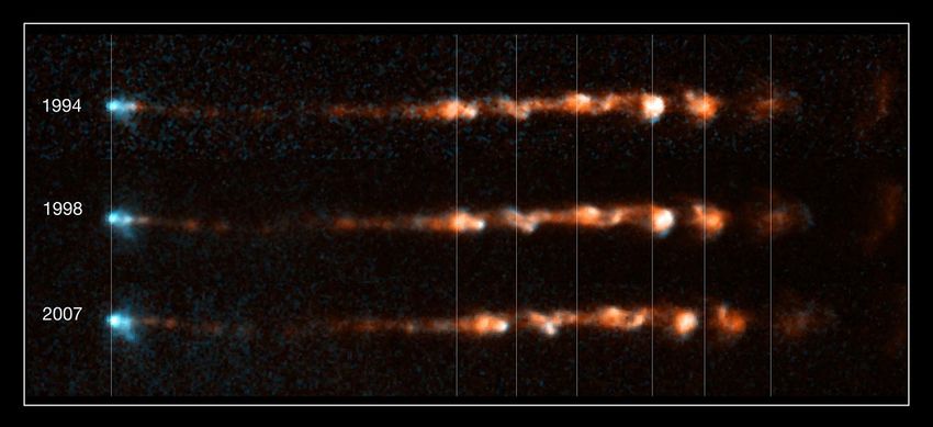
Abbildung 2 An ALMA image of the disk around the young star HL Tau. The image shows dust continuum emission.
Image from https://public.nrao.edu/static/pr/planet-formation-alma.html

Expected emission of a disk:
thin disk of surface density Σ( ) and temperature ( ) beginning at
radius 0 and extending up to radius 1
 projected ring area
dust opacity , inclination angle , received flux:
 2 cos 

 = ∫ Ω distance 
 Σ
 2 cos =
 
 = 2
 ∫ ( ) cos 
 = ( )[1 − − ]
 1
 2 cos 
 = ∫ ( ) [1 − exp (− )] 
 2 0 
Fitting an observation to the disk model requires Σ( ) and ( ) (and
 )

• complicated models of disk
 o temperature (heating, cooling)
 o density
 o chemical structure

Abbildung 3 Woitke et al. 2016

OPTICAL THICK LIMIT
 Σ
 = ≫ 1 ⇒ exp(− ) → 0
 cos 
Σ dependence removed in thick limit!
 4 cos ℎ 2 1 
 = ∫ 
 2 5 0 exp[ℎ /( )] − 1

ℎ 1/ 
assume = 0 ( / 0 )− and substitute = ( )
 0 0

 4 cos ℎ 2 0 2 1 
 = ( ) ∫ 
 2 5 0 0 exp[ ] − 1

 −2/ 1
 4 cos ℎ 2 ℎ 
 = ( ) ∫ 
 2 5 0 0 0 exp[ ] − 1

Integrating from 0 = 0 to 1 = ∞ ∝ (2−4 )/ 
At small wavelength this can be inverted and the temperature law can be
deduced.
OPTICAL THIN LIMIT
@long wavelengths (FIR, sub-mm), outer disk with lower Σ

 1 − exp (− )≈
 
 2 1
 = 2 ∫ ( ) 
 0
inclination becomes irrelevant. Assuming RJ limit
 2 
 ( ) ≈
 4
 4 _ 1
 = ∫ -dependence outside of
 2 4 0 integral
 assuming:

 ∝ − 
 ∝ −3− 

The sub-mm SED tells us about the wavelength dependence of the dust
opacity!

ISM: ≈ 2 in the diffuse ISM, ≈ 1 in the dense ISM
reduction in indicates grain growth
but also transition from optically thick to thin causes the SED to flatten!

11.1.3 Disks in molecular lines

Line emission also reveals kinematics!
e.g. truncation radius of disk from max. rotation velocity

Abbildung 4 Najita et al. 2007

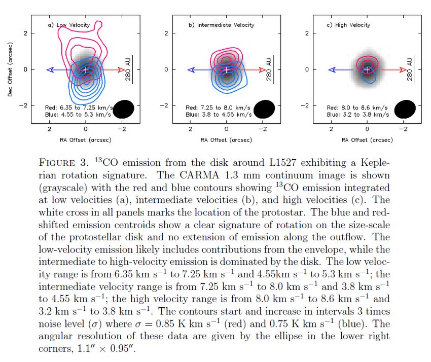
Abbildung 5 Tobin et al. 2012

Kepplerian orbits are fastest in the inner disk

11.2 OBSERVATIONS OF OUTFLOWS
11.2.1 Outflows in the optical

First detected in the optical in the 1950s (Herbig & Haro)
Small patches of optical emission (continuum & lines)
Interpretation: fast shock (-> ionization, therefore H emission) and
up/downstream we find neutral, warm material (emission lines)
1970: knots are aligned in linear structures (bi-polar) with bow shocks at
the head of the jets

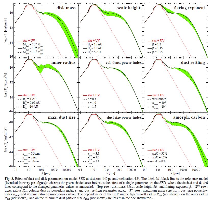
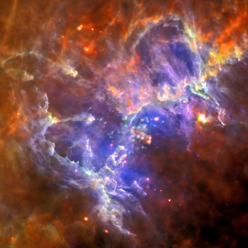
Abbildung 6 Herbig-Haro jets imaged with the Hubble Space Telescope.Two jets are visible; one is at the tip of the “pillar" near the
top of the image, and another is near the edge of the structure in the middle-left part of the image. Bow shocks from the jets are
clearly visible. Taken from http://hubblesite.org/newscenter/archive/releases/2010/13/image/a/.

knots: locations where the jet encountered a dense ISM region
(producing strong shocks) or where variations of the velocity or mass flux
feeding the jet caused internal shocks (then knots are symmetrically w.r.t.
to the both bipolar jets).
HH jets move typically with few 100s km s-1. Visible spatial variation on
timescales of 10 years.

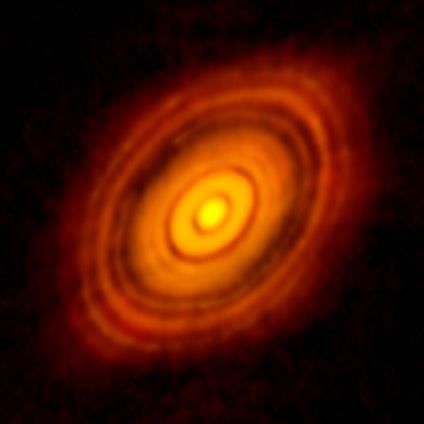
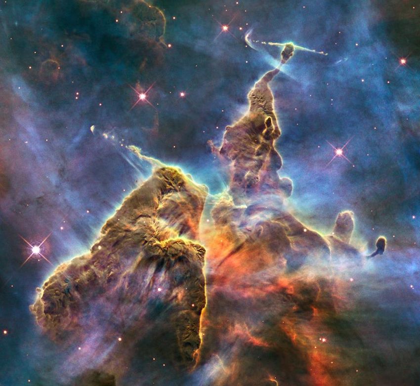
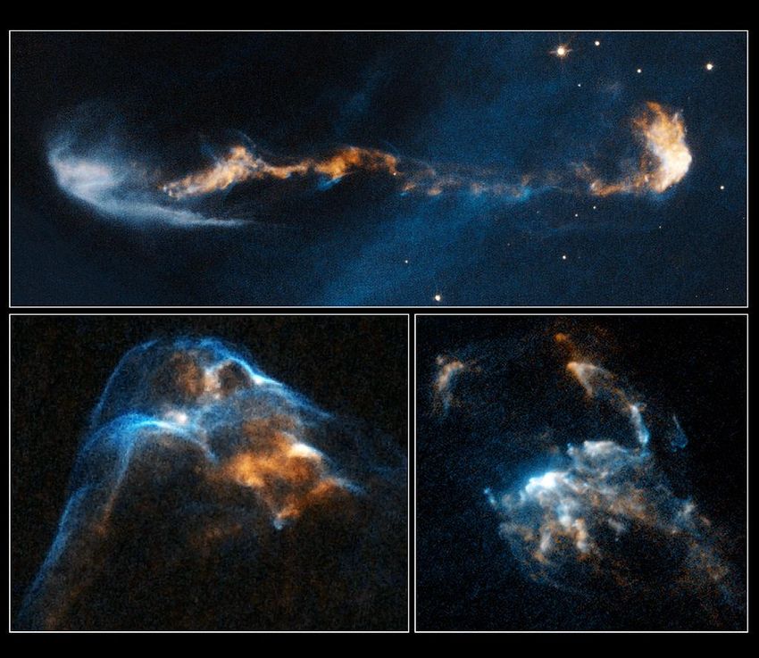
Abbildung 7 The glowing, clumpy streams of material shown in these NASA/ESA Hubble Space Telescope images are the signposts of
star birth. Ejected episodically by young stars like cannon salvos, the blobby material zips along at more than 700 000 kilometres per
hour. The speedy jets are confined to narrow beams by the powerful stellar magnetic field. Called Herbig-Haro or HH objects, these
outflows have a bumpy ride through space. When fast-moving blobs collide with slower-moving gas, bow shocks arise as the
material heats up. Bow shocks are glowing waves of material similar to waves produced by the bow of a ship ploughing through
water. In HH 2, at lower right, several bow shocks can be seen where several fast-moving clumps have bunched up like cars in a
traffic jam. In HH 34, at lower left, a grouping of merged bow shocks reveals regions that brighten and fade over time as the heated
material cools where the shocks intersect. In HH 47, at top, the blobs of material look like a string of cars on a crowded motorway,
which ends in a chain-reaction accident. The smash up creates the bow shock, left. These images are part of a series of time-lapse
movies astronomers have made showing the outflows’ motion over time. The movies were stitched together from images taken over
a 14-year period by Hubble’s Wide Field Planetary Camera 2. Hubble followed the jets over three epochs: HH 2 from 1994, 1997, and
2007; HH 34 from 1994, 1998, and 2007; and HH 47 from 1994, 1999, and 2008. The outflows are roughly 1350 light-years from
Earth. HH 34 and HH 2 reside near the Orion Nebula, in the northern sky. HH 47 is located in the southern constellation of Vela.

Estimated momentum flux: 10−6 − 10−3 M⊙ km s−1 yr −1 (very
uncertain)

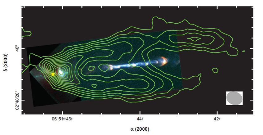
Abbildung 8 HH34, Credit: NASA, ESA, and P. Hartigan (Rice University)

11.2.2 Outflows in the radio

optical & near-IR: traces strong shock heating
molecular lines show that narrow optical jets are accompanied by a much
wider-angle, slower-moving and more massive molecular outflow

Abbildung 9 McKee & Ostriker 2007: The HH 111 jet and outflow system. The color scale shows a composite Hubble Space Telescope
image of the inner portion of the jet (WFPC2/visible) and the stellar source region (NICMOS/IR) (Reipurth et al. 1999). The green
contours show the walls of the molecular outflow using the v = 6 km s−1 channel map from the CO J = 1–0 line, obtained with BIMA
(Lee et al. 2000). The yellow star marks the driving source position, and the grey oval marks the radio image beam size; the total
length of the outflow lobe shown is ≈0.2 pc.

Molecular lines show: large masses of mol. gas moving at ~ 10 km s-1.
These component carry bulk of outflow momentum:
10−4 − 10−1 M⊙ km s−1 yr −1
Interpretation: not directly ejected material but ambient gas swept up by
the jets.

11.3 THEORY
11.3.1 Disk Formation
11.3.1.1 The Angular Momentum of Protostellar Cores

Measure the angular momentum by line observations:
Ω: angular velocity of the rotation, : moment of inertia of the core
ratio of in rotation to -> dimensionless measure 
 (1/2) Ω2 for sphere of uniform
 = density 
 2 / 
 1 2
 Ω2 3
 = Ω =
 4 3 
Typical observed values: few percent (Goodman et al. 1993)
Cores are not primarily supported by rotation
11.3.1.2 Rotating Collapse: The Hydrodynamic Case
Fluid element at distance from axis of rotation (assume in equatorial
plane)
Initial angular momentum: = 02 Ω (no pressure assumed)
Energy and j remains constant. At closest approach to central star its
velocity is max

 = √2 ∗ / , = 

 04 Ω2 4 04
 = =
 ∗ ∗
(radius at which infalling material must go into the disk because it cannot
come any closer)
 ∗ = (4/3) 03
 = 3 0
Cores of ~0.1 pc size should become rotationally flattened at radii of
several hundred AU

11.3.1.3 Rotating Collapse: The MHD Case

Effect of magn. fields: core contracts, rotation wants to spin up, twists
magn. field lines, tension force that opposes rotation and tries to keep
the core rotating like a solid body.

Cylindrical coordinates ( , , ), fluid element with velocity in 
direction
Magnetic field through fluid element: = ( , , )
poloidal component: = ( , ), toroidal component 
fluid and magn. field: axisymmetric
Lorentz force on fluid element poloidal gradient

 1 ∇ = ( / , / )
 = [(∇ × ) × ]
 4 
 1 ( ) 
 = [ + ] ̂
 4 
 1
 = ⋅ ∇ ( ) ̂
 4 
rate of change of momentum associated with the Lorentz force:
 
 ( ) = 
 

 component and multiplication with -> angular momentum
 1
 ( v ) = ⋅ ∇ ( )
 4 
left: time rate of change of angular momentum per unit volume 
right: torque per unit volume exerted by the magnetic field

magnetic braking time:
 ( v ) 4 v 
 ≈ =
 
 ( v ) ⋅ ∇ ( )
 
Consider a collapsing fluid element that is trying to rotate with Keplerian
velocity:

 = √ ≈ √(4 /3) 2
 
 (4 )3/2 1/2 2
 ≈
 ⋅ ∇ ( )
Assume: poloidal and toroidal components are comparable, characteristic
length scale on which field varies is , i.e. fairly smooth
Then
 ⋅ ∇ ( )~ 2 dropping all constants of
 order unity
 Alfven speed
 1/2 3/2 2 1/2 2 2
 ( ) = /√4 
 ~ ~ ~
 2 2 
 = / 

If the cloud starts with energetic equipartition: ~ 
so ~ 

Even a marginally wound up magn. field is capable of stopping Keplerian
rotation in a time scale comparable to the collapse or crossing time.
If the magn. field is strong enough this prevents disk formation at all!

11.3.1.4 The Magnetic Braking Problem

Problem: It naively seems like magnetic fields should prevent disks from
forming at all, but we observe that they do.
We even observe disks present in class 0 sources, where the majority of
the gas is still in the envelope.
 • Could Ion-Neutral drift offer a way out?
 o I-N-drift allows gas to decouple from magn. field on scales
 below ~0.05 . Disk formation below this scale?
 o Simulations suggest that this does not work.
 ▪ I-N drift -> gas flux released from the gas.

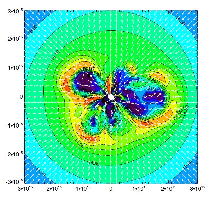
▪ I-N-drift builds up flux tubes near the star
 ▪ this flux tubes prevent disk formation

Abbildung 10 Results from a simulation of magnetized rotating collapse including the effects of ion-neutral drift and Ohmic
dissipation (Krasnopolsky et al., 2012). Lengths on the axes are in units of cm. Colors and contours show the density in the equatorial
plane, on a logarithmic scale from 10-16.5 to 10-12.5 g cm-3. Arrows show velocity vectors.

 • Misalignment between rotation axis and magnetic field
 o i.e. turbulence in the collapsing gas
 o turbulence bends and misaligns magnetic field lines
 o efficiency of magnetic breaking is greatly reduced
 • Problem still not fully solved

11.3.2 Disk Evolution
Given that disks exist, we wish to understand how they evolve, and how
they accrete onto their parent stars.
11.3.2.1 Steady Thin Disk

Consider: Thin disk ( = 0, only), Σ surface density, Ω angular velocity,
cylindrical symmetric (only function of radius )
orbital velocity = Ω, radial velocity (< , so gas can accrete)
equation of mass conservation:
 1 = Σ ( )
 + ∇ ⋅ ( ) = + ( ) = 0 drop components of
 
 divergence in and 
 1 directions
 Σ+ ( Σ ) = 0
 integrate over 
 1 
 Σ+ ̇ = 0 ̇ = −2 Σ 
 2 

 p: pressure
Navier-Stokes equation
 : grav. potential
 
 ( + ⋅ ∇ ) = −∇p − ρ∇ψ + ∇ ⋅ : viscous stress tensor
 
 integrate over 
 derivatives vanish
 1 2 because of symmetry
 Σ [ + ( )] = ∫ 2 ( ) 
 
 multiply by 2 2

 2πrΣ [ + ] = ∫ (2 2 ) = 
 
 = : angular
 momentum per unit
 mass
 = 2 ∫ 

2 Σ: mass per unit radius in a thin ring, 2 Σj: angular momentum in a
thin ring, : torque exerted on the ring due to viscosity.

Suppose we look for solutions of this equation in which the angular
momentum per unit mass at a given location stays constant: / = 0
This will be the case, for example, of a disk where the azimuthal motion is
purely Keplerian at all times. In this case the evolution equation just
becomes
 
 − ̇ =
 
the accretion rate ̇ is controlled by the rate at which viscous torques
remove angular momentum from material closer to the star and give it to
material further out.
In case of Keplerian rotation: = √ 
relationship: accretion rate-viscous torque
 • We will assume that the gas in the disk is Newtonian, meaning that
 the viscous stress is proportional to the rate of strain in the fluid.
 • We want to know , meaning the force per unit area in the 
 direction, exerted on the radial face of a fluid element.
 • Consider an observer in a frame comoving with the orbiting fluid at
 some particular distance r from the star
 • Consider a fluid element that is initially on the same radial ray as the
 observer, but a distance dr further from the star.
 • If the rotation is solid body, then the fluid element and the observer
 will always lie on the same radial ray, so there is no strain, and there
 will be no viscous stress.
 • If there is differential rotation, such that the fluid further the star
 has a longer orbital period (as we expect for Keplerian motion), the
 fluid element will gradually fall behind the observer. This represents
 a strain in the fluid.
How quickly does the element fall behind?
difference in angular momentum: Ω = ( Ω/ ) r
difference in spatial velocity: ( Ω/ ) r
rate of strain ( Ω/ ) / = ( Ω/ )

Viscous stress: rate of strain times the dynamic viscosity:
 Ω Ω kinematic viscosity
 = = 
 d d = / 

 Ω
 = 2 ∫ = 2 3 Σ 
 d 

Assume Keplerian rotation: = √ , Ω = √ / 3

 1 
 Σ− ̇ = 0
 2 
 
 − ̇ =
 
gives:
 Σ 3 1 1
 = [ 2 ( Σ 2 )]
 
 3 1
 = − 1 ( Σ 2 )
 
 Σ 2
 2
 ∝ 2 diffusion eq. , if we start with a sharply peaked Σ, say a surface
 
density that looks like a ring, viscosity will spread it out.
 Analytic solution for the viscous
 ring of material with constant
 kinematic viscosity . At time
 = 0, the column density
 distribution is Σ = Σ0 ( − 0 )
 Colored lines show the surface
 density distribution at later
 dimensionless times, as
 indicated in the legend. (Pringle
 (1981)).

How quickly to do rings spread, and does mass move inward?
Assume: Σ and are ~constant
 
 = −3 Σ 
 
 ̇ = 3 Σ 
 3 
 = −
 2 
The time required for a given fluid element to reach the star, therefore,
is:
 
 ~ ~ 2 / 
 
 Ω
 -Ansatz: = − Ω . It follows that
 dr

 2
 = = 
 Ω
 : sound speed, : disk scale height (both include thermal and magnetic
pressure).
 1 2
 = ( ) 
 
 1 2
Therefore, it takes about / = ( ) orbits to drain the disk!
 
Hartmann et al. (1998) estimate that ~10−2 in nearby T Tauri stars.
11.3.2.2 Physical Origins of Disk Viscosity

 • viscous mechanism to transport angular momentum and mass
 • estimated strength from observations
 • what mechanism?

ORDINARY FLUID VISCOSITY

Kinematic viscosity: = 2 ̅ ̅: RMS particle speed, : mean free path
protostellar accretion disk:
 = 1012 −3 , = 100 , ̅ = 0.6 −1 ,
 1
 = (1 )2 , = = 100 , ~108 −2 
 
Let us consider material at a temperature of 100 K that is orbiting 100 AU
from a 1 ⊙ star.
 = 0.6 −1 , Ω = 6.3 × 10−3 −1 => ≈ 6 × 10−12 (!)
Suppose the gas starts out ~100 AU from the star. The time required for
the gas to accrete is then
 2 (100 )2
 ~ ~ ~1022 ~1015 
 
Longer than universe!
If that were the only source of angular momentum transport in a disk,
then stars would never form. Something else must be at work.
TURBULENT HYDRODYNAMICAL VISCOSITY
If there are large-scale radial motions within a disk, then the effective
value of ̅ could be significantly larger than the microphysical one we
calculated. In effect, these motions will mix material from different radii
within the disk, exchanging angular momentum between inner and outer
parts of the disk.
Numerical simulations have been attempted, and seem to find that
hydrodynamic mechanisms do not produce significant angular
momentum transport, but they may be compromised by limited
resolution.
Laboratory experiments can reach Reynolds numbers of ~106, and seem
to find negligible transport < 10−6 (Ji et al., 2006). Given these results,
most researchers are convinced that purely hydrodynamic mechanisms
cannot explain the observed lifetimes and rates of angular momentum
transport in disks. Instead, some other mechanism is required.
MAGNETO-ROTATIONAL INSTABILITY

• The basic idea is that magnetic field lines threading the disk connect
 annuli at different radii.
 • As the disk rotates and the annuli shear, this stretches the magnetic
 field line connecting them.
 • This causes an opposing magnetic tension, which attempts to force
 the two points to stay close together, and thus to force them into
 co-rotation.
 • This speeds up the outermost fluid element, which is falling behind,
 and slows down the innermost one, and thus it moves angular
 momentum outward.
 • However, when you remove angular momentum from a fluid
 element it tends to fall toward the center, so the innermost fluid
 element falls even closer to the star.
 • Similarly, the outermost fluid element gains angular momentum,
 and so it wants to move outward.
 • This increases the tension even more, and the system goes unstable
 due to this positive feedback loop.
Simulators are still working to try to come up with a general result about
the value of produced by the MRI, but in at least some cases a as high
as 0.1 seems to be possible.
Problem:
 • MRI will only operate as long as matter is sufficiently coupled to the
 magnetic field
GRAVITATIONAL TRANSPORT MECHANISMS
Gravitational Instability: Toomre parameter :
 3 3
 ̇ =
 
If > 1 (grav. stable), and < 1 maximum rate at which the disk can
move matter ~ 3 / .
This is also the characteristic rate at which matter falls onto the disk from
a thermally-supported core, provided that we use the sound speed in the
core rather than in the disk.

 in any regions where the disk is not significantly warmer than the
 core that is feeding it (e.g. the outer parts of the disk where stellar
 and viscous heating are small), the disk cannot transport matter
 inward as quickly as it is fed.
  the surface density will rise and Q will decrease, giving rise to
 gravitational instability.
  This can in turn generate transport of angular momentum via
 gravitational torques.
  The disk can also transfer angular momentum to the star by forcing
 the star to move away from the center of mass. In this configuration
 the disk develops a one-armed spiral, and the star in effect goes into
 a binary orbit with the over-density in the disk.
  This phenomenon is known as the Sling instability Shu et al. (1990).

11.3.3 Outflow Launching
How and why disks launch the ubiquitous jets and winds that
observations reveal.
Driving mechanism?
Stellar winds?
 • High pressure in solar corona drives gas outward: mechanical
 luminosity: ~10−4 ⊙
 • Observed outflows from young stars: ~0.1 ⊙
 • No!
Photon pressure?
 • stellar photon field does not have enough momentum to drive the
 observed outflows of young stars
Neither the thermal winds of low mass main sequence stars, nor the
radiatively-driven winds of massive ones, show highly collimated features
like the HH jets.
Most natural mechanism: gravitational potential energy being liberated
by the accretion flow, which, combined with magnetic fields, can produce
highly collimated outflows.