Stress Field of a Rectangular Dislocation Loop - Asee peer logo

Paper ID #35154

Stress Field of a Rectangular Dislocation Loop
Mr. Luo Li, University of New Mexico
 I am Luo Li and I am a graduate student from UNM. I am currently working with Dr.Tariq Khraishi. We
 published a paper ’The Strain/Stress Fields of a Subsurface Rectangular Dislocation Loop Parallel to the
 Surface of a Half Medium: Analytical Solution with Verification’ in Jamp. Now, we are wokring on the
 paper ’Stress Field of a Rectangular Dislocation Loop’. I hope I can investigate more problems in the
 future.
Prof. Tariq Khraishi, University of New Mexico
 Khraishi currently serves as a Professor of Mechanical Engineering at the University of New Mexico. His
 general research interests are in theoretical, computational and experimental solid mechanics and mate-
 rials science. He has taught classes in Dynamics, Materials Science, Advanced Mechanics of Materials,
 Elasticity and Numerical Methods. For many years now, he has engaged himself in the scholarship of
 teaching and learning, and published several papers in the engineering education field.

 c American Society for Engineering Education, 2021

1

 The Stress Field of a Rectangular Dislocation Loop

 Luo Li
 Mechanical Engineering Department
 University of New Mexico
 Albuquerque, NM 87131
 luol@umm.edu

 Tariq Khraishi
 Mechanical Engineering Department
 University of New Mexico
 Albuquerque, NM 87131
 khraishi@umm.edu

 Abstract
Dislocations are line defects in crystals and they possess a displacement, strain and stress fields
associated with them. Much research has gone into determining these fields as the understanding of
dislocations is fundamental to understanding metal or crystal plasticity. In this paper, the stress field
of a rectangular dislocation loop in an infinite isotropic solid is developed here for a Volterra-type
dislocation with three non-zero Burgers vector components. To be specific, the stress field of the
dislocation loop in an infinite isotropic material is obtained by integrating the Peach-Koehler equation
over a rectangular perimeter. In this paper, analytical and numerical verifications of the developed
stress field are performed. This is done by ensuring the satisfaction of the equilibrium equations and
the strain compatibility equations. Furthermore, a comparison with the stress field of a Volterra-type
dislocation loop composed of four dislocation segments, using DeVincre’s formula, is presented. The
results of this paper add to the knowledge base of elastic fields of dislocation loops which has
applications in plasticity modeling, fracture mechanics, etc.

 Introduction
Dislocations are line defects, around which the atoms of the crystal lattice are misaligned. There are
two basic types of dislocations, the edge dislocation and screw dislocation. For a rectangular
dislocation closed loop, there are four linear dislocation segments. Dislocation lines have to end on
free surfaces or grain boundaries or form a close loop inside a material instead of ending inside the
material1. Moreover, a dislocation loop with the Burgers vector parallel to the plane of the loop is
called a Glide dislocation loop. However, Prismatic dislocation loops are with a Burgers vector
normal to the plane of the loop. In this paper, the stress field of a Volterra-type rectangular dislocation
loop, which has three Burgers vector components bx, by, bz, is developed. A Volterra dislocation is one
where the Burgers vector does not change magnitude or direction along the dislocation line with
respect to an inertial coordinate system.

Three-dimensional dislocation dynamics codes2,3 rely on fundamental dislocation solutions like the
one presented in this paper. Such codes or simulations can capture the plasticity behavior of an
ensemble of dislocations in a computational domain. In these codes, a continuously curved dislocation
 Proceedings of the 2021 ASEE Gulf-Southwest Annual Conference
 Baylor University, Waco, TX
 Copyright  2021, American Society for Engineering Education

2

line in 3D is discretized in one form or another. The stress field of the original dislocation curve is
provided by the sum of the stress fields of dislocation segments composing the curve. This is from the
principle of linear superposition. The self-stress of a straight dislocation segment of mixed character
has been provided prior in the literature4.

Different kinds of dislocation problems in terms of material type, geometry and size have been
investigated for tens of years. Derivations for the displacement, strain and stress fields of screw and
edge dislocations in an infinite medium, assuming material isotropy, were presented5,6,7. Moreover,
integral equations for finding the displacement field (the Burgers equation) and the stress field of a
closed dislocation loop (of any shape) in an infinite isotropic material have also been provided5.

In this paper, the stress field of a rectangular dislocation loop in an infinite isotropic material is
developed by integrating the Peach-Koehler equation over the perimeter of a finite rectangular
dislocation loop. Also, analytical and numerical verifications for the stress solution obtained herein
are presented. Furthermore, a comparison with the stress field of a rectangular loop composed of four
dislocation segments, applying the DeVincre formula4, is presented. For a semi-infinite material on
the other hand, a recent solution was presented8 for the stress and strain fields of a rectangular
dislocation loop that is beneath and parallel to the free surface.

In addition to the utility of the presented solution for dislocation dynamics codes, such fundamental
dislocation solutions are also needed for the “distributed dislocation method” used to solve fracture or
crack problems. It also has utility in general eigenstrain problems9,10. Lastly, they can play a role in
“collocation-point” methods used in conjunction with free surfaces11-16.

 Method
In this paper, the dislocation problem under consideration is shown in Figure 1. The figure shows a
rectangular dislocation loop of finite-size in an unbounded isotropic solid. This Volterra-type
dislocation loop has three Burger vector components bx, by and bz, and has a dimension 2a in the x-
direction and a dimension 2b in the y-direction. The vector around the loop sides shows the line sense
of the dislocation. The goal of this paper is to obtain the stress field at an arbitrary material point P
shown in Figure 1, as mentioned in the Introduction. Note that, 1 and x are used interchangeably, so
are 2 and y, and so on. Similarly for ′1 and ′, and so on.

 Proceedings of the 2021 ASEE Gulf-Southwest Annual Conference
 Baylor University, Waco, TX
 Copyright  2021, American Society for Engineering Education

3

 Figure 1. The figure of a rectangular dislocation loop in infinite material. Note that ⃗ ′ = ′ =
 ( ′ , y ′ , z ′ ) and that z ′ = .

The Peach-Koehler Equation, equation (1), is an integral equation for the stress field of any curved
and closed dislocation loop5. It is formed by three terms: they are all line integrals summing the
contributions of infinitesimal line lengths ( ′) forming the loop along its line sense:

 = − ∮ ′ ∇′2 ′ − 8 ∮ ′ ∇′2 ′ −
 8 
 3 ′2 ′
 ∮ ( ′ 
4 (1− ) ′ ′
 − 
 ′
 ∇ ) ; (1)
 
, where is the ℎ component of the stress vector ⃗, is the mth component of the Burgers
vector ⃗⃗ = = ( , , ), is the th component of the Kronecker delta, is shear
modulus, ∈ is the permutation symbol, is Poisson’s ratio, =
 2
√( ′ − )2 + ( ′ − )2 + ( ′ − )2 (see Figure 1) and ∇′ = 2/ . Note that, bold and top
arrow placement are both used interchangeably for a vector quantity. (e.g. ⃗⃗ = )

For the integration of Peach-Koehler Equation, some steps need to be considered. Firstly, the
elevation of the dislocation loop is fixed in the global coordinate system ( , , ), which means
 ′ = 0 or the value of ′ is constant in this case. Secondly, ′ is a constant equal to + along
 Proceedings of the 2021 ASEE Gulf-Southwest Annual Conference
 Baylor University, Waco, TX
 Copyright  2021, American Society for Engineering Education

4

segment 1, which means ′ = 0 along this segment. Analogously, ′ = − and ′ = 0 along
segment 3, ′ = + and ′ = 0 along segment 2, ′ = − and ′ = 0 along segment 4. For
brevity, only the integration for for a non-zero is presented as an example of the
integration of the Peach-Koehler Equation.

 3 3 
 = ∮ ( ′ ′ ′) ′ − 4 (1− ) ∮ ( 2 ′ ′) ′ =
 4 (1− ) 
 + 3 − 3 
{ ∫ [( ′ ′ ′) ′ ] ′ =+ } + {4 (1− ) ∫+ [( ′ ′ ′) ′ ] ′=− } −
 4 (1− ) − 
 − 3 + 3 
{ ∫ [( 2 ′ ′) ′ ] ′=+ } − {4 (1− ) ∫− [( 2 ′ ′) ′ ] ′=− };
 4 (1− ) + 
 (2)

 + 3 
Let’s take −{ ∫ [( 2 ′ ′) ′ ] ′=− } as an integration example.
 4 (1− ) − 

 3 3(− + ′ )2 (− + ′ ) − + ′
 = 5⁄2
 − .
 2 ′ ′ ((− + ′ )2 +(− + ′ )2 +(− + ′ )2 ) ((− + ′ )2 +(− + ′ )2 +(− + ′ )2 )3⁄2

If one is interested in integrating the last integral by hand, one can use integral tables17. Since
 + 3 
there are two integrals for the integration −{ ∫ [( 2 ′ ′) ′ ] ′=− , which are
 4 (1− ) − 
 2
 + 3(− + ′ ) (− + ′ )
−{ ∫ [(((− + ′)2+(− + ′)2+(− + ′)2)5⁄2) ′ ] ′=− } and
 4 (1− ) − 
 + − + ′
−{ ∫ [(− ((− + ′ )2+(− + ′)2+(− + ′)2)3⁄2) ′ ] ′=− } respectively. Only the second
 4 (1− ) − 
 + − + ′
integral −{ ∫ [(− ((− + ′)2+(− + ′)2+(− + ′)2)3⁄2) ′ ] ′=− =
 4 (1− ) − 
 + − + ′
{ ∫ [(((− + ′ )2+(− + ′)2+(− + ′)2)3⁄2) ′ ] ′=− } is shown here.
 4 (1− ) − 
 2(2 + )
According to the integral table17, ∫ = , (3)
 √ 1 3 (4 − 2 )√ 1

where 1 = + + 2 ;
 − + ′ − + ′
Note that 3⁄2
 can be written as 2 .
 ((− + ′ )2 +(− + ′ )2 +(− + ′ )2 ) ( ′ −2 ′ + 2 +(− + ′ )2 +(− + ′ )2 )3⁄2
 2 2
In this example, 1 = ′ − 2 ′ + 2 + (− + ′ )2 + (− + ′ )2 = + ′ + ′ , where
 = 2 + (− + ′ )2 + (− + ′ )2, = −2 , = 1.
According to equation (3),
 − + ′ (− + ′ ) ′ 2(2 ′ + )(− + ′ )
∫ 2 ′ = ∫ = =
 ( ′ −2 ′ + 2 +(− + ′ )2 +(− + ′ )2 ) 3⁄2
 √ 1 3 (4 − 2 )√ 1

 2(2 ′ −2 )(− + ′ )
 =
 2
(4( 2 +(− + ′)2 +(− + ′ )2 )−4 2 )√ ′ −2 ′ + 2 +(− + ′ )2 +(− + ′ )2
 Proceedings of the 2021 ASEE Gulf-Southwest Annual Conference
 Baylor University, Waco, TX
 Copyright  2021, American Society for Engineering Education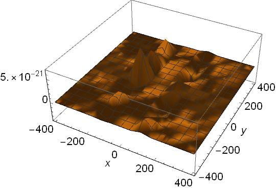

5

 ( ′ − )(− + ′ )
 ;
 ((− + ′ )2 +(− + ′ )2 )√(− + ′ )2 +(− + ′)2 +(− + ′ )2

 + − + ′
 Hence, ∫ [(((− + ′)2+(− + ′)2+(− + ′ )2)3⁄2) ′ ] ′=− =
 4 (1− ) − 
 ( − )(− + ′ )
 {[ ]−
 4 (1− ) ((− − )2 +(− + ′ )2 )√(− + )2 +(− − )2 +(− + ′ )2
 (− − )(− + ′ )
 [ ]}; (4)
 ((− − )2 +(− + ′ )2 )√(− − )2 +(− − )2 +(− + ′ )2

 Alternatively, one can also use the mathematical software Mathematica, which has a very strong
 symbolic engine, to do the integrations. This is a more efficient process. In this paper, all the
 integrations and solutions are obtained using Mathematica.

 Results and Discussion
The stress field of a rectangular dislocation loop in an infinite medium was developed utilizing the
mathematical software Mathematica. The stress results are listed in the Appendix for a non-zero bx.
For non-zero by or bz, the results of the integration are not provided herein for brevity. If one is
interested instead in the strain components at an arbitrary field point, these can be obtained from
stresses using Hooke’s law:
 1
 = ((1 + ) − ) (5)
, where, is the th component of the strain tensor, is the first invariant of the stress tensor, 
is the th component of the Kronecker delta, is Poisson’s ratio, is Young’s modulus.

Equilibrium Equations Verification
The partial differential equations of static equilibrium in a solid material can be written via equations
(6)-(8):
 
 + + =0 (6)
 
 + 
 + 
 =0 (7)
 
 + + =0 (8)
 
These equations should be satisfied at every material point of a solid in equilibrium. To verify the
developed stress solution given by equation (1), one can see if equations (6-8) are identically zero
either using analytical or numerical methods. For the analytical method, the equations are all
converted to zero using Mathematica. Hence analytical verification of the equilibrium equations is
completed.

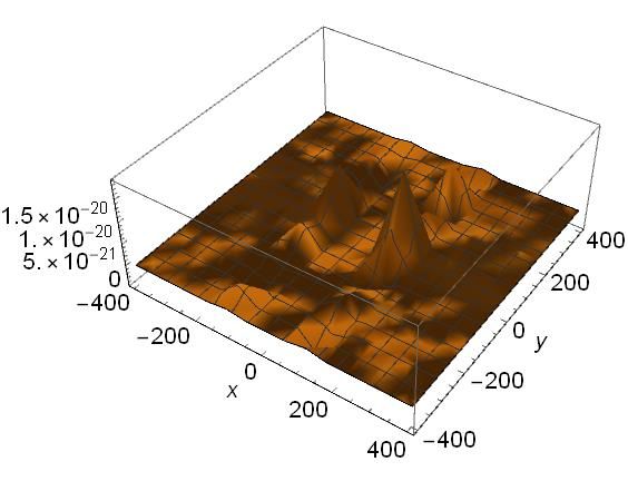
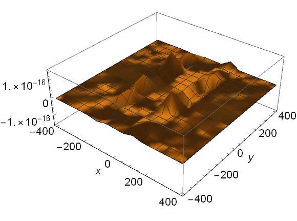
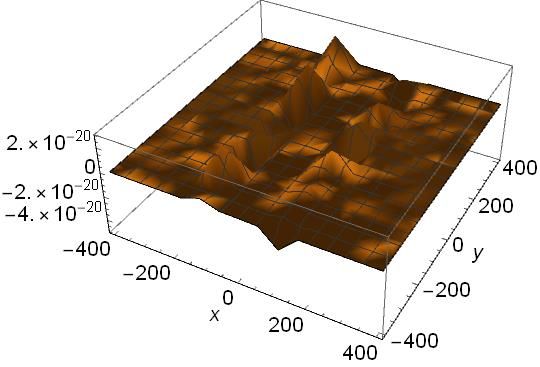
Alternatively, numerical verifications can also be carried by plotting equations (6)-(8) along any plane
in the material to see if the equations present a zero result. Figure 2 shows such plotting for bz ≠ 0.
The figure shows that the equilibrium equations are satisfied. Note that given the combination of
Burgers vector components and equilibrium equations, a total of nine plots are minimally generated.
For brevity, only three plots for one of the Burgers vector components are shown here.

 Proceedings of the 2021 ASEE Gulf-Southwest Annual Conference
 Baylor University, Waco, TX
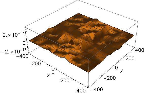
 Copyright  2021, American Society for Engineering Education

6

Figure 2.1. Plot of equation (6) showing satisfaction of the equation

Figure 2.2. Plot of equation (7) showing satisfaction of the equation

Figure 2.3. Plot of equation (8) showing satisfaction of the equation

For these plots, the following values were chosen: = = 100 , = 10 , = = 0, = 1,

 Proceedings of the 2021 ASEE Gulf-Southwest Annual Conference
 Baylor University, Waco, TX
 Copyright  2021, American Society for Engineering Education

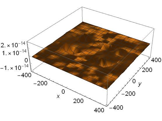
7

 = 0.3, = = 100, = 11 , −4 ≤ ≤ 4 , −4 ≤ ≤ 4 

Strain Compatibility Equation Verification
The equations of compatibility can be written explicitly as six different and unique equations18:
 2 2 2 2 2 2 
 
 + = 2 (9) + = 2 (10)
 2 2 2 2
 2 2 2 2 2 2 2 
 + = 2 (11) + = + (12)
 2 2 2 
 2 2 2 2 2 2 2 2 
 + = + (13) + = + (14)
 2 2 
These equations should be satisfied at every material point of a solid. To verify the developed stress
solution, one can utilize strain compatibility equations, where the strain field is given by equation (5).
Then, one can see if equations (9)-(14) are identically zero either using analytical or numerical
methods. For the analytical method, the equations are so large that Mathematica is not able to convert
them to 0. However, for any given line in space along the x-, y- or z-directions, Mathematica
identically simplifies the strain compatibility equations to zero. Hence, analytical verification of the
compatibility equations is possible.
Alternatively, numerical verification can also be made by plotting equations (9)-(14) along any plane
in the material to see if the equations give a zero result. Figure 3 shows such plotting for bx ≠ 0, which
presents that the compatibility equations are satisfied. Note that given the combination of Burgers
vector components and compatibility equations a total of eighteen plots are minimally generated.
However, only three plots for one of the Burgers vector components are shown here for brevity.

Figure 3.1. Plot of equation (9) showing satisfaction of the equation

 Proceedings of the 2021 ASEE Gulf-Southwest Annual Conference
 Baylor University, Waco, TX
 Copyright  2021, American Society for Engineering Education

8

Figure 3.2. Plot of equation (10) showing satisfaction of the equation

Figure 3.3. Plot of equation (11) showing satisfaction of the equation.
 For these plots, the following values were chosen: = = 100 , = 10 , = = 0, = 1,
 = 0.3, = = 100, = 11 , −4 ≤ ≤ 4 , −4 ≤ ≤ 4 

DeVincre’s Formula Verification
The DeVincre’s Formula4 is the expression for the stress field of a straight dislocation segment, which
is restricted to linear isotropic elasticity. This formula is given in tensor and vector notation expressed
with respect to an arbitrary Cartesian reference frame. Furthermore, this solution is able to compute
the self-stress field of a dislocation segment. A curved dislocation line can be approximated by
continuous linear dislocation segment. In order to use this formula, one needs the line sense of the
dislocation segment, its Burgers vector, the coordinates of the two end points of the segment, the
shear modulus and Poisson’s ratio.
In this paper, the rectangular dislocation loop is composed of four straight dislocation segments (these
are the four sides of the rectangular loop in Figure 1). Hence, the stress field of a rectangular
dislocation loop at any field point is the sum of the stresses from the four segments. To compare the
current solution with the stress field solution obtained from DeVincre’s Formula, the following
parameters were used for plotting purposes (Figures 4-6):
 = = 100 , = 0, = 0.3, = = 100, = = 0; = 1; = 0, z = 20 , −2 ≤ ≤
 Proceedings of the 2021 ASEE Gulf-Southwest Annual Conference
 Baylor University, Waco, TX
 Copyright  2021, American Society for Engineering Education

9

2 .
The figures show almost perfect match between the analytical solution in this paper and the solution
obtained from DeVincre’s Formula. Note that given the combination of Burgers vector components
and stress components, a total of eighteen plots are minimally generated. However, only three plots
for one of the Burgers vector components are shown here for brevity. Although the exact behavior of
stress in these figures for these chosen points in space is not important, however, the figures show
some expected results. For example, the stress decays towards zero away from the dislocation line.
Also, the stress is high in vicinity of the dislocation line.

Figure 4.

Figure 4. Comparison of analytical solutions in this paper (solid black line) to the results of the
 
DeVincre’s Formula (dashed line) along y-direction for with non-zero by.

Figure 5.

Figure 5. Comparison of analytical solutions in this paper (solid black line) to the results of the
 Proceedings of the 2021 ASEE Gulf-Southwest Annual Conference
 Baylor University, Waco, TX
 Copyright  2021, American Society for Engineering Education

10

DeVincre’s Formula (dashed line) along y-direction for with non-zero by.
 
Figure 6.

Figure 6. Comparison of analytical solutions in this paper (solid black line) to the results of the
 
DeVincre’s Formula (dashed line) along y-direction for with non-zero by.

 Conclusions
In conclusion, the analytical solution for the stress field associated with a rectangular dislocation loop
in infinite material has been developed. It was obtained by integrating the Peach-Keohler equation
over a finite rectangular dislocation loop. Moreover, the strain field can also be obtained from the
stress using Hooke’s law. Such fundamental solution can have several applications as mentioned in
the Introduction. The developed stress field was verified both numerically and analytically. This was
done against the equilibrium equations, compatibility equations and DeVincre’s Formula.

 References
1. Meyers, M.A., Chawla, K.K., 2009, Mechanical Behavior of Materials, 2nd ed. University of Cambridge, UK.
2. Rhee, M., Zbib, H.M., Hirth, J.P., Huang, H., Dela-Rubia, T., 1998, “Modelling Simul Mater”, Sci. Engng,
Vol. 6, No. 4, pp. 467-492.
3. Zbib, H.M., Rhee, M., Hirth, J.P., 1998, “On plastic deformation and the dynamics of 3D dislocations”, Int.
 J. Mech. Sci., Vol. 40, No. 2-3, pp. 113-127.
4. DeVincre, B., 1995, “Three dimensional stress field expressions for straight dislocation segments”,
Solid State Communication, Vol. 93, No. 11, pp. 875-878.
5. Hirth, J.P., Lothe, J., 1982, Theory of Dislocations, 5th ed. Krieger Publishing Company,
Malabar, Florida.
6. Hull, D., Bacon, D.J., 2011, Introduction to Dislocations, University of Liverpool, UK.
7. Weertman, J., Weertman, J.R., 1992, Elementary Dislocation Theory, University Press, Oxford.
8. Li, L., Khraishi, T.A., Siddique, A.B., 2021, “The Strain/Stress Fields of a Subsurface Rectangular
Dislocation Loop Parallel to the Surface of a Half Medium: Analytical Solution with Verification”, Journal of
Applied Mathematics and Physics, Vol. 9, No.1, pp. 146-175.
 Proceedings of the 2021 ASEE Gulf-Southwest Annual Conference
 Baylor University, Waco, TX
 Copyright  2021, American Society for Engineering Education

11

9. Lerma, J.D., Khraishi, T.A., Shen, Y.L., 2007, “Elastic Fields of 2D and 3D Misfit
Particles in an Infinite Medium”, Mechanics Research Communications, Vol. 34, No. 1, pp. 31-43.
10. Lerma, J., Khraishi, T., Kataria, S., Shen, Y.-L., 2015, “Distributed Dislocation Method for Determining
Elastic Fields of 2D and 3D Volume Misfit Particles in Infinite Space and Extension of the Method for Particles
in Half Space,” Journal of Mechanics, Vol. 31, Issue 3, pp. 249-260.
11. Khraishi, T.A., Zbib, H.M., De La Rubia, T.D., 2001, “The Treatment of Traction free Boundary Condition
in Three-dimensional Dislocation Dynamics using Generalized Image Stress Analysis,” Materials Science and
Engineering A, Vol. 22, pp. 283-287.
12. Khraishi, T.A., Zbib, H.M., 2002, “Free Surface Effects in 3D Dislocation Dynamics: Formulation and
Modeling,” Journal of Engineering Materials and Technology (JEMT), Vol. 23, pp. 342-351.
13. Yan, L., Khraishi, T.A., Shen, Y.-L., Horstemeyer, M.F., 2004, “A Distributed Dislocation Method for
Treating Free-Surface Image Stresses in 3D Dislocation Dynamics Simulations,” Modelling and Simulation in
Materials Science and Engineering, Vol. 24, pp. 289-301.
14. Siddique, A.B., Khraishi, T.A., 2020, “Numerical methodology for treating static and dynamic dislocation
problems near a free surface,” Journal of Physics Communications, Vol. 1, 055005, DOI 10.1088/2399-
6528/ab8ff9.
15. Siddique, A.B., Khraishi, T.A., 2021, “A Mesh-Independent Brute-Force Approach for Traction-Free
Corrections in Dislocation Problems”, Modeling and Numerical Simulation of Material Science, Vol. 11, No.01,
pp. 1-18.
16. Siddique, A.B., Khraishi, T.A., 2021, “Screw Dislocations Around Voids of Any Shape: A Generalized
Numerical approach”, Forces in Mechanics, Vol. 3, 100014, https://doi.org/10.1016/j.finmec.2021.100014
17. Gradshteyn, I.S., Ryzhik, I.M., 1980, Table of Integrals, Series, and Products, 5th ed. Academic Press: San
 Diego, California.
18. Khraishi, T.A., Shen, Y.L., 2011, Introductory Continuum Mechanics with Applications to Elasticity,
University Readers/Cognella, San Diego, California.

 Appendix
Below are the stress components as a function of the isotropic material constants and spatial coordinate for the case of a
non-zeor bx. For the other Burgers vector components, the results are not provided here for brevity.

σ b ( − ) + − + 
 = 2(( − )2 +( − )2 )(−1+ ) (
 − )+
 √( − )2 +( − )2 +( + )2 √( − )2 +( − )2 +( − )2
 b ( − ) + − + 
 (− + )+
2(( − ) +( + )2 )(−1+ ) 
 2 √( − )2 +( + )2 +( + )2 √( − )2 +( + )2 +( − )2
 b ( − ) 2 2 2
 (( − ) +( − ) )( − ) ( + ) (( − )2 −( − )2 )( + )
 (
4(( − )2 +( − )2 )2 (−1+ ) (( − )2 +( − )2 +( + )2 )3⁄2
 − −
 √( − )2 +( − )2 +( + )2
(( − )2 +( − )2 )( − )2 (− + ) (( − )2 −( − )2 )(− + )
 + )+
 (( − )2 +( − )2 +( − )2 )3⁄2 √( − )2 +( − )2 +( − )2
 b ( − ) ((( − )2 +( + )2 )( + )2 −(( − )2 +( + )2 +( + )2 )(( − )2 −( + )2 ))( + )
 (− +
4(( − )2 +( + )2 )2 (−1+ ) (( − )2 +( + )2 +( + )2 )3⁄2
((( − ) +( + ) )( + ) −(( − ) +( + ) +( − ) )(( − )2 −( + )2 ))(− + )
 2 2 2 2 2 2
 );
 (( − )2 +( + )2 +( − )2 )3⁄2
σ b ( − ) 1 ( + ) (− + )
 = ((−1+ ) (− (( − )2 +( − )2 +( + )2 )3⁄2 + (( − )2 +( − )2 +( − )2 )3⁄2 ) +
 4 
 2 + (− + )
 ( − )+
(( − )2 +( − )2 )(−1+ ) √( − )2 +( − )2 +( + )2 √( − )2 +( − )2 +( − )2
 1 + (− + )
 ( − (( − )2 +( + )2 +( − )2 )3⁄2 ) +
(−1+ ) (( − )2 +( + )2 +( + )2 )3⁄2
 2 + (− + )
 (− + )+
(( − )2 +( + )2 )(−1+ ) √(( − )2 +( + )2 +( + )2 ) √( − )2 +( + )2 +( − )2
 1 + (− + )
2((( − )2 +( − )2 ) ( − )+
 √( − )2 +( − )2 +( + )2 √( − )2 +( − )2 +( − )2

 Proceedings of the 2021 ASEE Gulf-Southwest Annual Conference
 Baylor University, Waco, TX
 Copyright  2021, American Society for Engineering Education

12

 1 + (− + )
 (− + )));
(( − )2 +( + )2 ) √( − )2 +( + )2 +( + )2 √( − )2 +( + )2 +( − )2
σ b ( − ) + (− + )
 = 2(( − )2 +( − )2 )(−1+ ) ( − )+
 √( − )2 +( − )2 +( + )2 √( − )2 +( − )2 +( − )2
 b ( − ) + (− + )
 (− + )+
2(( − )2 +( + )2 )(−1+ ) √( − )2 +( + )2 +( + )2 √( − )2 +( + )2 +( − )2
 b ( − ) (−(( − )2 +( − )2 )( − )2 +(( − )2 +( − )2 +( + )2 )(( − )2 +3( − )2 ))( + )
 (− +
4(( − )2 +( − )2 )2 (−1+ ) (( − )2 +( − )2 +( + )2 )3⁄2
(−(( − )2 +( − )2 )( − )2 +(( − )2 +( − )2 +( − )2 )(( − )2 +3( − )2 ))(− + )
 )+
 (( − )2 +( − )2 +( − )2 )3⁄2
 b ( − ) (−(( − )2 +( + )2 )( − )2 +(( − )2 +( + )2 +( + )2 )(( − )2 +3( + )2 ))( + )
 ( −
4(( − )2 +( + )2 )2 (−1+ ) (( − )2 +( + )2 +( + )2 )3⁄2
(−(( − )2 +( + )2 )( − )2 +(( − )2 +( + )2 +( − )2 )(( − )2 +3( + )2 ))(− + )
 );
 (( − )2 +( + )2 +( − )2 )3⁄2
σ b ( − ) 1 1
 = 4(−1+ ) ((− (( − )2 +( − )2 +( − )2 )3⁄2 + (( − )2 +( − )2 +( + )2 )3⁄2 )( − ) +
 
 1 1
(− (( − )2 +( + )2 +( − )2 )3⁄2 + (( − )2 +( + )2 +( + )2 )3⁄2 )( + )) +
b ( − ) 1 ( − ) ( + )
 (( − )2 +( − )2 (− − )+
 4 √( − )2 +( − )2 +( − )2 √( − )2 +( + )2 +( − )2
 1 ( − ) ( + )
 ( + ));
( − )2 +( + )2 √( − )2 +( − )2 +( + )2 √( − )2 +( + )2 +( + )2
σ b ( − ) (( − )2 +( − )2 )( − )2 (( − )2 −( − )2 )
 = 4(( − )2 +( − )2 )2 (−1+ ) (−(− (( − )2 +( − )2 +( + )2 )3⁄2 − )( + ) +
 √( − )2 +( − )2 +( + )2
 (( − )2 +( − )2 )( − )2 (( − )2 −( − )2 )
(− (( − )2 +( − )2 +( − )2 )3⁄2 − )(− + )) +
 √( − )2 +( − )2 +( − )2
b 1 ( − ) ( + )
 ( ( + )( + ) −
4 ( − )2 +( + )2 √( − )2 +( − )2 +( + )2 √( − )2 +( + )2 +( + )2
 1 ( − ) ( + )
 ( + )(− + )) +
( − )2 +( − )2 √( − )2 +( − )2 +( − )2 √( − )2 +( + )2 +( − )2
 b ( + ) (( − ) +( + )2 )( − )2
 2 (( − )2 −( + )2 )
 (( + )( + ) +
4(( − )+( + )2 )2 (−1+ ) (( − )2 +( + )2 +( + )2 )3⁄2 √( − )2 +( + )2 +( + )2
 (( − )2 +( + )2 )( − )2 (( − )2 −( + )2 )
(− (( − )2 +( + )2 +( − )2 )3⁄2 − )(− + ));
 √( − )2 +( + )2 +( − )2
σ b 1 1 1
 = 4 ( − − +
 √( − )2 +( − )2 +( − )2 √( − )2 +( − )2 +( + )2 √( − )2 +( + )2 +( − )2
 1 1 ( − )2 +( + )2 ( + )2 +( + )2
 + (−1+ ) (− (( − )2 +( − )2 +( + )2 )3⁄2 + (( − )2 +( + )2 +( + )2 )3⁄2 +
√( − )2 +( + )2 +( + )2
 ( − )2 +(− + )2 ( + )2 +(− + )2
 − (( − )2 +( + )2 +( − )2 )3⁄2 ));
(( − )2 +( − )2 +( − )2 )3⁄2

LUO LI
Luo Li is a graduate student in the Mechanical Engineering Department at the University of New Mexico. He is currently
studying for his MSME. In his undergraduate program, Mr Luo Li was engaged in CAD, 3D printing and finite-element
analysis. His Bachelor degree’s graduation project was on finite-element analysis of linear friction welding. For his
Masters degree, he is focused on solid mechanics and materials science/engineering. He already has two journal papers
published and a third under review.

TARIQ A. KHRAISHI
Khraishi currently serves as a Professor of Mechanical Engineering at the University of New Mexico. His general research
interests are in theoretical, computational and experimental solid mechanics and materials science. He has taught classes
in Dynamics, Materials Science, Advanced Mechanics of Materials, Elasticity and Numerical Methods. For many years
now, he has engaged himself in the scholarship of teaching and learning and published several papers in the engineering
education field.
 Proceedings of the 2021 ASEE Gulf-Southwest Annual Conference
 Baylor University, Waco, TX
 Copyright  2021, American Society for Engineering Education