Supplement of Optimized Umkehr profile algorithm for ozone trend analyses
←
→
Page content transcription
If your browser does not render page correctly, please read the page content below
Supplement of Atmos. Meas. Tech., 15, 1849–1870, 2022
https://doi.org/10.5194/amt-15-1849-2022-supplement
© Author(s) 2022. CC BY 4.0 License.

Supplement of
Optimized Umkehr profile algorithm for ozone trend analyses
Irina Petropavlovskikh et al.

Correspondence to: Irina Petropavlovskikh (irina.petro@noaa.gov)

The copyright of individual parts of the supplement might differ from the article licence.
S1. Umkehr biases and time series for OHP, MLO and Lauder

     This section shows comparisons of the operational (Fig. S1), SLC (Fig. S2) and optimized (Fig. S3) versions of Umkehr
     records from OHP, MLO and Lauder against multiple independent records during the 2005-2020. The biases between
     operationally processed Umkehr data and other records (including ozonesonde station records) are similar in vertical
 5   distribution (i.e. large positive biases in the upper and middle stratosphere and negative biases in the UTLS) to the results of
     Boulder Umkehr record. A large noticeable bias between M2GMI and GMI CTM ozone profiles is found at Lauder station in
     the lower stratosphere (layers 4, 3 and 2). The SLC versions of the Umkehr data at three stations (Fig. S2) show reduction in
     biases in the upper stratosphere similar to the changes found in Boulder record (Fig. 5a). This reduction in upper layer biases
     is accompanied by changes in the biases in the lower layers, especially in layer 2 (decrease), 3 (increase for OHP and Lauder)
10   and layer 4 (increase for MLO and Lauder).
     After the optimization (Fig. S3), a significant reduction in biases is found in layers 4-9 with the exception of comparisons at
     Lauder where M2GMI bias has become more negative, but still less than 5 %, which is within the uncertainty of the Umkehr
     retrieval. At the same time, the M2GMI bias in layer 2 increased to 5 % at OHP and less than 5 % at MLO, which is similar
     to the bias between ozonesonde and optimized Umkehr. The Lauder station features a negative bias between the optimized
15   Umkehr and ozonesonde data in layers 2 and 3, while a positive bias of similar magnitude is found at OHP. No significant
     biases are found in comparisons of MLO optimized Umkehr with Hilo ozonesonde data. The Hilo ozonesonde profiles are
     limited to the pressure level above 680 hPa, which is the surface pressure at MLO.
     The Umkehr and COH comparisons in layer 2 and 3 at all three stations show small and positive biases (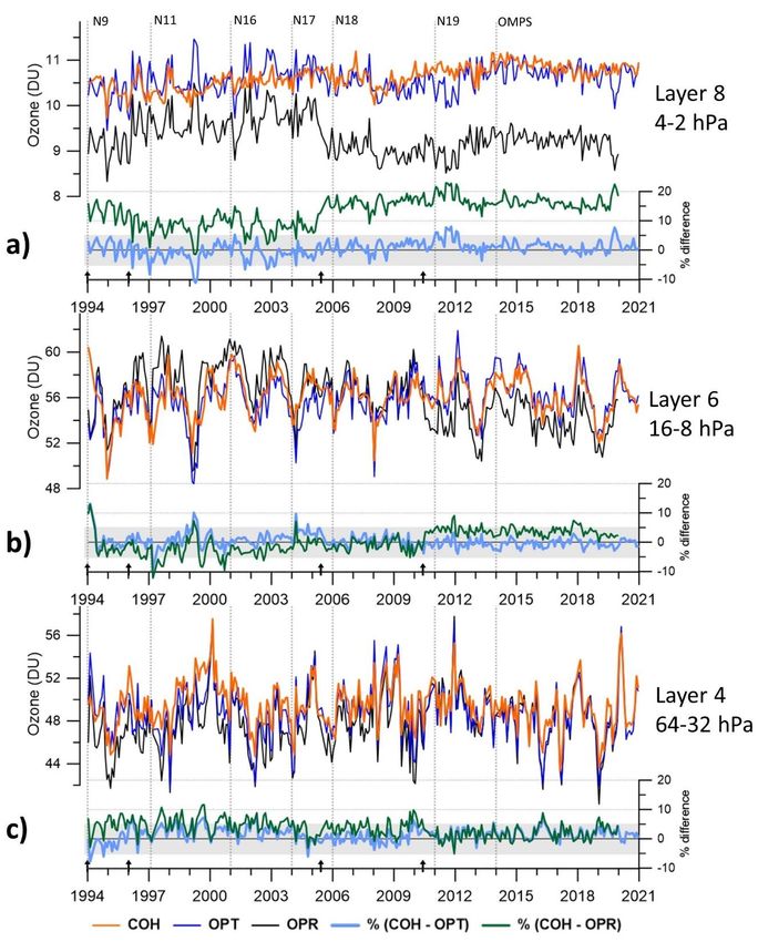
layer 6 and layer 4 shows the smallest impact of the optimization process as expected from the vertical contribution of the out-
     of-band errors.
35   The temperature related step-change in the upper stratosphere in the MERRA-2 assimilations is reflected in both M2GMI and
     GMI CTM models (Stauffer et al, 2019 and references therein). The step change in MERRA-2 is from the addition of MLS
     temperature to the observing system starting in 2004. Ozone chemical timescales are short in the upper stratosphere, so any
     transport induced changes have little to no impact on ozone. However, temperature impact kinetic reactions rates. Therefore,
     the step change in assimilated temperatures creates a step-change in stratospheric ozone.
40   To assess the impact of the 2004/2005 step-change in the M2GMI and GMI CTM records (Stauffer et al, 2019) on Umkehr
     optimization and homogenization process we plot biases for 1994-2004 and 2005-2020 periods (Fig. S10). Based on these
     comparisons, we notice that the biases between M2GMI and Umkehr are reduced by 2 % in the upper stratosphere in 2005-
     2020 period, whereas relative biases between M2GMI and GMI CTM are contained. Similar changes in the upper stratospheric
     biases between the M2GMI and optimized Umkehr for two analysed periods are found for Boulder (Fig. 5a), although the
45   absolute biases are different. The 2005-2020 period shows an improved agreement between Umkehr and M2GMI record, as
     well as bias between Umkehr and COH record is reduced below 20 hPa, except there is no reduction with respect to the GMI
     CTM bias. The differences in stratospheric ozone offsets between ozonesonde/M2GMI (smaller) and ozonesonde/GMI (larger)
     over Lauder were reported in Stauffer et al. (2019) paper and had similar range of biases derived in this study at the lower and
     middle stratosphere.
50   In conclusion, the optimization reduces biases between Umkehr ozone profiles and most of the alternative coincident records
     to less than +/- 5 % at all four stations. Investigation of large biases between GMI CTM and other records at Lauder needs
     further investigation.

     S2. Umkehr optimization for volcanic time periods.

     During the volcanic eruptions (like El Chichon in 1982 or Pinatubo in 1991) sulphate aerosols were ejected to stratosphere and
55   were transported globally or semi-globally. The large amounts of aerosol load, as large as to 0.1 in optical depth in UV
     wavelengths (Stevermer et al, 2000), significantly contributed to the scattered light in the atmosphere. Figure S11, panel a
     shows two large deviations during the volcanic period in the apparent transmission time series measured at MLO. While the
     operation Umkehr ozone retrieval algorithm does not account for aerosol-produced scatter in its forward model, and therefore
     interprets changes in observed N-values as changes in ozone profile. This creates a period of erroneous ozone values. Figure
60   B1, panel b, shows the reduced ozone in stratospheric layer 8 of the MLO operational Umkehr record (black line). The most
     depleted ozone is found soon after the eruption, coincident with the largest aerosol load, and then the error in retrieved ozone
     is slowly reduced following a decay in aerosol particles over ~2-year time period.
     The optimization to remove the low bias in the Umkehr ozone profile during volcanic periods is performed following a similar
     approach as discussed in this paper, except the corrections are developed for several 6-month long incremental periods. The

                                                                    2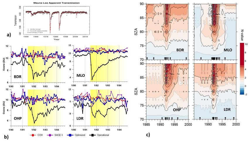
65   result is shown in Panel b with a blue line. For the reference, the M2GMI data are also shown (red line) and compare well with
     the optimized Umkehr results. Yet as an independent reference the SAGE II data are also shown for comparisons (purple line).
     Volcanic corrections to the Umkehr N-values are presented in panel c of Figure S11 for three stations (Boulder, OHP, MLO
     and Lauder) as function of SZA and time. The timing of the volcanic aerosol transport and decay can be discerned at tropical
     latitude locations as captured in the Umkehr record at MLO in 1991-1993. While in the northern middle latitudes (Boulder or
70   OHP) the aerosols appear to be still impacting Umkehr observations at large SZAs until 1997, and in the southern hemisphere
     (Lauder) until 1999.

     S3. Umkehr Averaging Kernel

     Table C1 summarizes the Umkehr layer system. Each Umkehr layer is defined by the pressure at the bottom of the layer. The
     highest layer extends to the top of the atmosphere. The standard Umkehr output is constructed in 10-layer system (2 left-most
75   columns in Table C1). The 16-layer system (two middle columns in Table C1) is used for the AK output. The 61-layer system
     (two right-most columns in Table C1) is the working grid of the Umkehr retrieval algorithm to avoid interpolation errors
     (Petropavlovskikh et al., 2005).
     Figure S12 shows Umkehr Averaging Kernels (AK) as function of pressure and respective Umkehr layers (as defined in Table
     C1). The 61-, 16- and 10-layer AKs are shown in panels a, b, and c respectively. The AK concept is described by Rodgers
80   (2000). For plotting purposes, we follow Bhartia et al. (2013) formulation of the “smoothing” kernels that act as the low-pass
     filters to smooth fractional anomalies in each layer. The Fig. S12 shows the rows of the fractional AK that indicate the
     sensitivity of the retrieved ozone at that layer to changes in ozone at all layers. The red/green colors (see legend in panel a)
     highlights the high/low informational content of the AK. The maximum AK values between ~100 and 2 hPa are aligned with
     the nominal altitude of the layer, indicating the highest informational content obtained from that layer, while contribution from
85   adjacent layers is reduced at an exponential rate. Below 100 hPa (and above 2 hPa) level the maximum of the AK is shifted
     higher (lower) in altitude and the AK becomes broader. This means that the retrieval is the most sensitive to the ozone
     variability in the above (below) layers and therefore relies more heavily on the a priori information in order to separate
     informational content into individual layers. The Umkehr ozone profile is reported in 10 layers selected such that the
     informational content is provided at about two datapoints per width of the smoothing kernel. The vertical resolution at the
90   bottom of the profile is poor and therefore several layers are combined into a thicker layer that represents tropospheric column
     ozone information (see Table C1).

     S4. Temperature sensitivity in Umkehr retrievals

     The UMK08 operational algorithm (Petropavlovskikh et al. 2005) is based on the Bass and Paur (BP) ozone cross-section
     (Bass and Paur, 1985), convolved over the Dobson C-pair standardized band-pass (Komhyr et al, 1993; Petropavlovskikh

                                                                    3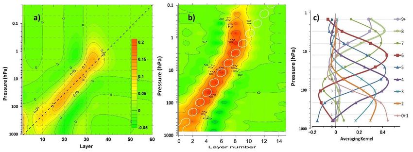
95   et. al, 2011). The impact of the ozone cross-section on the uncertainty of Brewer- and Dobson-observed total column ozone
      retrieval was outlined in detail by Redondas et al. (2014). They found that the use of Serdyuchenko et al. (2014) cross-section
      reduces the bias between Dobson and Brewer total column ozone observations and also reduces the temperature-dependent
      biases. An ad hoc commission of the Scientific Advisory Group (SAG) of the Global Atmosphere Watch (GAW) of the World
      Meteorological Organization (WMO) and the International Ozone Commission IO3C) of the International Association of
100   Meteorology and Atmospheric Sciences (IAMAS) performed the assessment of different ozone cross-section spectral
      databases and their temperature dependence (Orphal et al., 2016). For operational Umkehr retrievals, the effects of the ozone
      cross-section were found to be minimal (less than 2 %) when NRL (Summers and Sawchuck, 1993) climatological
      temperatures were used in the retrieval. However, the report suggests the use of the Serdyuchenko et al. (2014) ozone cross-
      sections in Umkehr retrievals whenever total ozone is processed with that cross-section. It is also suggested that day-to-day
105   and diurnal variability in stratospheric temperatures is larger than represented by climatology and thus may add additional 1-
      2 % change in daily stratospheric ozone that is not currently captured by operational Umkehr retrievals.

      The nominal absorption cross-sections for the WMO GAW Dobson total ozone network are derived based on the selection of
      a standardized temperature −46.3 ◦C (Komhyr et al, 1993, Redondas et al, 2014). The previously published approach to
110   represent temperature sensitivity in ozone absorption cross section (i.e. Redondas et al, 2014 and references within) is to use
      a second-degree polynomial in temperature. We use a spectrally resolved dataset (Bass and Paur, 1984; Serdyuchenko et al,
      2014) to calculate the effective ozone absorption cross-sections and their temperature dependence for C-pair spectral channels.
      Next section shows examples of Umkehr retrieved ozone sensitivity to the variability in ozone absorption cross section. Table
      S2 provides coefficients for second-degree polynomials fitted to the Bass and Paur (1984) absorption cross sections over
115   spectral bands of Dobson Umkehr C-pair (short and long) (Redondas et al., 2014).
      Figure S13 shows a change in Umkehr layer 8 ozone (4-2 hPa) as a function of temperature. The blue dots represent changes
      derived from the polynomial fit (Table D1). The dark circle shows the averaged ozone change associated with replacing
      standard temperature with the effective temperatures calculated from the subset of the GMI CTM temperature and ozone
      profiles matched to Boulder, CO location and selected for 2005-2018 period (GMIave). The red circle represents results based
120   on the mean temperature from the NRL climatology, 35-46 N (NRLav (N40)), Finally, the dark purple circle shows results
      based on the ML Climatology at 40 degrees N (McPeter and Labow, 2012). The horizontal whiskers represent a range of
      seasonal variability in temperature weighted by ozone profiles (between -30 and -12 degrees C) that results in layer 8 ozone
      changes between -4 and +2 %.
      We further assess the representativeness of the NRL temperature climatology used in the operational Umkehr algorithm. We
125   compare the temperature seasonal cycle derived from the M2GMI dataset over the Boulder station to the NRL climatology at
      40 degrees N over the 2010-2017 time period (Figure S14a). Monthly averaged M2GMI temperatures at 2.8 hPa are shown
      for the morning (red symbols and lines) and afternoon (grey symbols and lines) Umkehr measurements (i.e. at 15 UTC or 08
      LT, and 03 UTC or 20 LT). The NRL temperature climatology is shown for comparison (blue crosses). The day-to-day

                                                                    4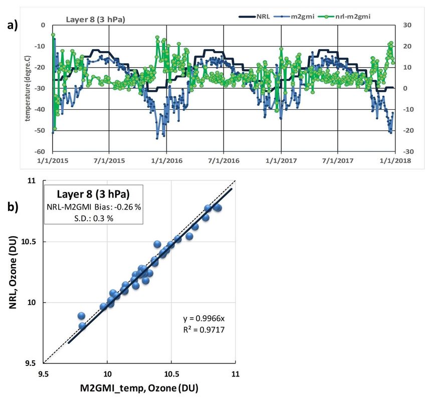
variability in M2GMI temperatures are shown as whiskers (the minimum and maximum of all data, one standard deviation
130   above and below the mean of the data). Figure 4a shows that the NRL climatology mean temperature is biased higher in the
      morning than in the afternoon by ~8.9 and 6.3 K respectively, which is an indication of the diurnal cycle at 2.8 hPa that is not
      captured by the NRL climatology). Also, day-to-day variability in the stratospheric temperature (see Figure S14b, results are
      based on M2GMI temperature dataset) can create an offset that varies seasonally (i.e. box and whiskers values). The summer
      months show less variability in daily temperatures as compared to the winter months, where maximum offset can vary between
135   -5 and 20 degrees C from the NRL climatological.
      Impact of daily temperature variability on retrieved Umkehr ozone profiles are further tested for 2015-2017 Boulder Umkehr
      record. Figure S15 shows M2GMI daily and NRL monthly temperatures at 2.8 hPal. The difference in temperatures during
      days when Umkehr observations were made is also plotted and highlights large deviations in the winter months. This day-to-
      day temperature variability as high as 20 degrees results in relatively low ozone variability. The changes in the retrieved ozone
140   are based on temperature sensitivity in the spectrally resolved ozone cross section within Dobson spectral channels and profile
      smoothing. Panel b of Figure 5 shows comparisons between ozone retrieved using NRL climatology (y-axes) and M2GMI
      daily temperature profiles (X-axes). Each point is monthly averaged ozone for 2015-2017 time period. The solid line is the 1:1
      reference. The mean bias is -0.26 % with 0.3 % standard deviation. This test provides an averaged uncertainty of the daily
      retrieved Umkehr ozone in layer 8. It may be a small error; however, this additional uncertainty varies from year to year and
145   thus can have an impact on the long-term ozone trend results in the upper stratosphere.

      References
      Bass A.M., and R.J. Paur, The ultraviolet cross-sections of ozone: I. The measurements in Atmospheric ozone (Ed. C.S.
      Zerefos and A. Ghazi), Reidel, Dordrecht, Boston, Lancaster, pp. 606-610, 1985.
150   Bhartia, P. K., McPeters, R. D., Flynn, L. E., Taylor, S., Kramarova, N. A., Frith, S., Fisher, B., and DeLand, M.: Solar
      Backscatter UV (SBUV) total ozone and profile algorithm, Atmos. Meas. Tech., 6, 2533–2548, https://doi.org/10.5194/amt-
      6-2533-2013, 2013.
      Komhyr, W. D., Mateer, C. L., & Hudson, R. D., Effective Bass-Paur 1985 ozone absorption coefficients for use with Dobson
      ozone spectrophotometers. Journal of Geophysical Research, 98(D11), 20451–20465, doi: 10.1029/93JD00602
155   McPeters, R. D., and Labow, G. J. (2012), Climatology 2011: An MLS and sonde derived ozone climatology for satellite
      retrieval algorithms, J. Geophys. Res., 117, D10303, doi:10.1029/2011JD017006.
      Orphal, J, J. Staehelin, J. Tamminen, G. Braathen, et al.: “Absorption cross-sections of ozone in the ultraviolet and visible
      spectral regions: Status report 2015”, Journal of Molecular Spectroscopy, Volume 327, 2016, Pages 105-121, ISSN 0022-
      2852, https://doi.org/10.1016/j.jms.2016.07.007, 2016.
160   Petropavlovskikh, I., Evans, R., McConville, G., Oltmans, S.,Quincy, D., Lantz, K., Disterhoft, P., Stanek, M., and Flynn,
      L.: Sensitivity of Dobson and Brewer Umkehr ozone profile retrievals to ozone cross-sections and stray light effects,
      Atmos. Meas. Tech., 4, 1841–1853, doi:10.5194/amt-4-1841-2011, 2011.

                                                                     5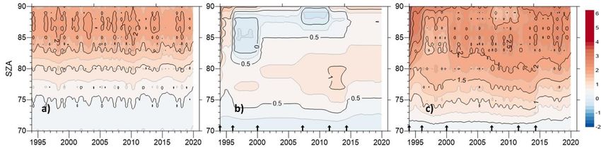
Redondas, A., Evans, R., Stuebi, R., Köhler, U., and Weber, M.: Evaluation of the use of five laboratory-determined ozone
      absorption cross sections in Brewer and Dobson retrieval algorithms, Atmos. Chem. Phys., 14, 1635–1648, doi: 10.5194/acp-
165   14-1635-2014, 2014.
      Serdyuchenko, A., Gorshelev, V., Weber, M., Chehade, W., and Burrows, J. P.: High spectral resolution ozone absorption 540
      cross-sections –Part 2: Temperature dependence, Atmos. Meas. Tech., 7, 625–636, https://doi.org/10.5194/amt-7-625-10 2014,
      2014.
      Stauffer, R. M., Thompson, A. M., Oman, L. D., & Strahan, S. E.: The effects of a 1998 observing system change on MERRA‐
170   2‐based ozone profile simulations. Journal of Geophysical Research: Atmospheres, 124, 7429–7441, doi:
      10.1029/2019JD030257, 2019.
      Stevermer, A. J., Petropavlovskikh, I. V., Rosen, J. M., and DeLuisi, J. J., Development of a global stratospheric aerosol
      climatology:   Optical   properties   and   applications   for       UV,   J.   Geophys.   Res.,   105   (D18),   22763–22776,
      doi:10.1029/2000JD900368, 2000.
175   Summers, M. E. and Sawchuck, W.: Zonally Averaged Trace Constituent Climatology. A Combination of Observational Data
      Sets and 1-D and 2-D Chemical-Dynamical Model Result, Naval Research Laboratory, Technical Report, NRL/MR/7641-93-
      7416, Washington, DC, 1993.

180

185

                                                                       6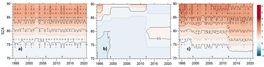
190
195
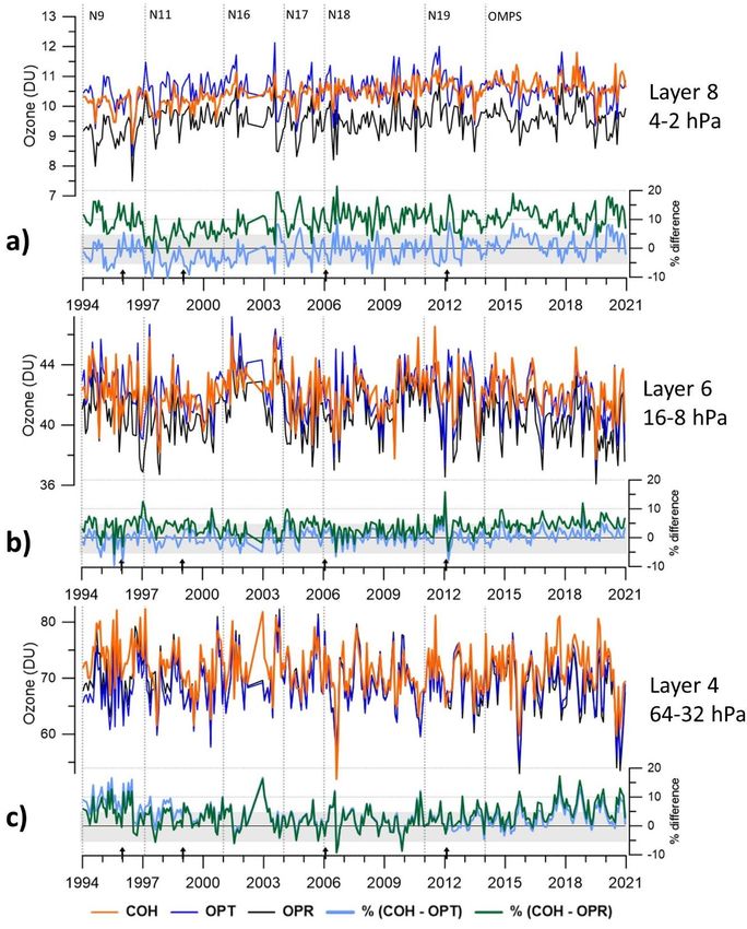
Figure S1. The same as right panel of Figure 1a, but for three other Umkehr records: OHP (left), MLO (middle) and Lauder (right).
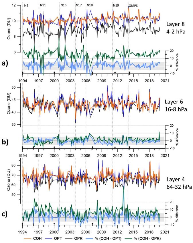
Figure S2. The same as right panel of Figure 1b, but for three other Umkehr records: OHP (left), MLO (middle) and Lauder (right).
200
7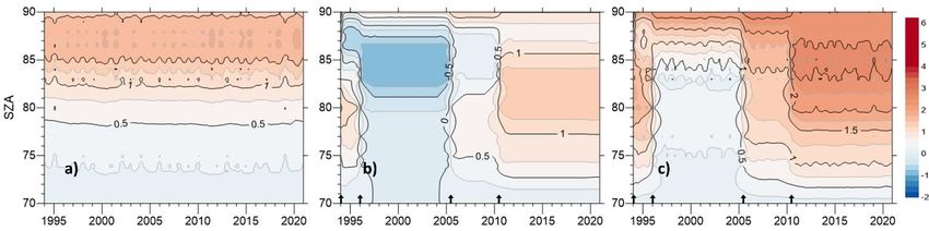
Figure S3. The same as the right panel of Figure 5a, but for three other Umkehr records: OHP (left), MLO (middle) and Lauder
      (right).

205

      Figure S4. Same as Fig. 3, but for OHP.

210   Figure S5. Same as Fig. 3, but for MLO.

                                                                   8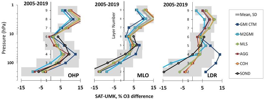
Figure S6. Same as Fig. 3, but for Lauder.

                                             9
215
Figure S7. Same as Fig. 7, but for the OHP record.
10220 Figure S8. Same as Fig, 7, but for the MLO record.
11Figure S9. Same as Fig, 7, but for the Lauder record.
12Figure S10. Same as Figure 5a, but for the Lauder station.
225
13Figure S11. Corrections derived for Boulder, OHP, MLO, and Lauder Umkehr operational ozone records during the period of
enhanced stratospheric aerosol load after the Pinatubo eruption in 1991. a) MLO record shows reduced apparent transmission after
1991 volcanic eruption (https://www.esrl.noaa.gov/gmd/grad/mloapt.html), b) ozone monthly mean time series in layer 8 (DU) from
230 Umkehr operational (black line), Umkehr optimized (blue), COH (red) and SAGE II (purple) records. The four panels show ozone
records compared at Boulder (BDR), MLO, OHP and Lauder (LDR) stations. The yellow shaded area indicates the period of the
enhanced volcanic aerosol load in the stratosphere. The black line shows an abrupt reduction in operational Umkehr ozone records
starting in the middle of 1991, followed by a gradual increase in ozone until 1994. The blue line (OPT, corrections applied) shows no
decline in layer 8 ozone during volcanic eruption, similarly to SAGE II records. c) same as Figure 8c, but during the Pinatubo
235 eruption. Arrows at the bottom of the panels indicate dates of Dobson calibrations.
14Figure S12. Umkehr Averaging Kernel (AK) is shown for Umkehr retrieval in layers with a) fine vertical resolution (forward model
grid, pressure on the y axes is matched to the sub-layer number, roughly every four sub-layers form one nominal Umkehr layer, see
Table 4) b) AKs for 16-layers, white circles imply a 1:1 line, c) AKs for 10-layers (optimized for independent information content in
240 10 nominal Umkehr layers). Colors in panel a) represent the weights of AK for each layer, where orange color represents the
maximum (typically centered at the diagonal) and green color is used for the minimum (can be a small negative number within the
uncertainty of the a priori). Colors in Panel c correspond to 10 Umkehr layers (See Table 4). The AKs are shown as an example,
they were taken from the operational (UMK04) ozone profile derived on March 2, 2018, at Boulder station.
245
Figure S13. Change in Umkehr layer 8 ozone as function of temperature estimated from the second-degree polynomial fit (see
coefficients in Table D1). The blue dots represent the range of middle latitude temperature variability, the grey circle shows mean
effective temperature based on 2005-2020 GMI CTM over Boulder, CO (GMIave), the red circle is the mean 35-46 N NRL
temperature climatology, marked as NRLav (N40) in the legend. The dark purple circle is the mean climatological temperature at
250 40-45 N (McPeter and Labow, 2011) and whiskers represent a range of seasonal variability in temperature and ozone over Boulder,
CO at 4-2 hPa layer and during 2005-2020 period.
15Figure S14. a) Seasonal difference between NRL and M2GMI monthly averaged over 2010-2017 time period and selected at 15 UTC
and at 2.8 hPa pressure level (Umkehr layer 8). b) the same as a), but time is at 3 UTC.
255
16Figure S15. Impact from the NRL climatology and M2GMI temperature on ozone variability in Umkehr layer 8 (3 hPa) at Boulder
station. a) Time series of temperature. b) Ozone derived with temperature correction based on the NRL and M2GMI data. A dashed
line is 1:1 slope, a solid line is the linear fit. The bias and standard deviation are shown in the box in the upper left corner, the slope
260 and correlation coefficient are shown in the lower right corner.
17265 Table S1. Umkehr and COH pressure layer grids. The layer is defined by the pressure at the bottom of the layer. The pressure at
the top layer is between the pressure level and the top of the atmosphere. The standard Umkehr output is in 10-layer system (2
leftmost columns). The 16-layer system (columns 3 and 4) is used for the AK output. The 61-layer system (columns 5 and 6) is utilized
in the forward model. The COH 21-layer system (columns 7 and 8) is the standard output. All COH profiles are interpolated to the
10- or 61- layer Umkehr grid for intercomparisons.
270
Table S2. Wavelengths and temperature coefficients for the second-degree polynomial fit, calculated using B&P ozone cross section
data and weighted with C-pair handpasses.
275
18You can also read