Supplement of Sensitivity to the sources of uncertainties in the modeling of atmospheric CO2 concentration within and in the vicinity of Paris
←
→
Page content transcription
If your browser does not render page correctly, please read the page content below
Supplement of Atmos. Chem. Phys., 21, 10707–10726, 2021
https://doi.org/10.5194/acp-21-10707-2021-supplement
© Author(s) 2021. CC BY 4.0 License.

Supplement of
Sensitivity to the sources of uncertainties in the modeling of atmospheric
CO2 concentration within and in the vicinity of Paris
Jinghui Lian et al.

Correspondence to: Jinghui Lian (jinghui.lian@suez.com)

The copyright of individual parts of the supplement might differ from the article licence.
Supplement

      Figure S1: Time series of average CO2 concentration differences between CAMS and CarbonTracker at four lateral boundaries (west,
 5    east, south, north), averaged over vertical layers above 0.7 km AGL, of D01 for 00 UTC in blue and 12 UTC in red. The lines indicate
      the spatial means over each boundary (a latitudinal transect for western and eastern boundaries / a longitudinal transect for southern
        and northern boundaries). The shaded areas extend over one standard deviation (± 1σ) computed over the grid cells that make the
     lateral boundary (spatial standard deviation). The yellow symbols indicate the days when the wind blows from outside of the domain at
      the respective domain boundary. The numbers on the right side of the figure indicate annual means of (i) the spatial mean and (ii) the
10                                                           spatial standard deviation.

                                                                                                                                          1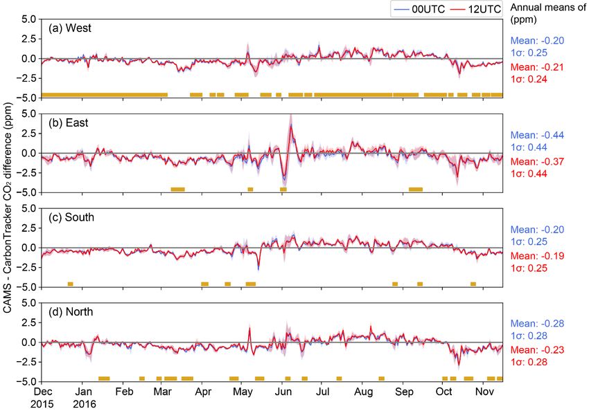
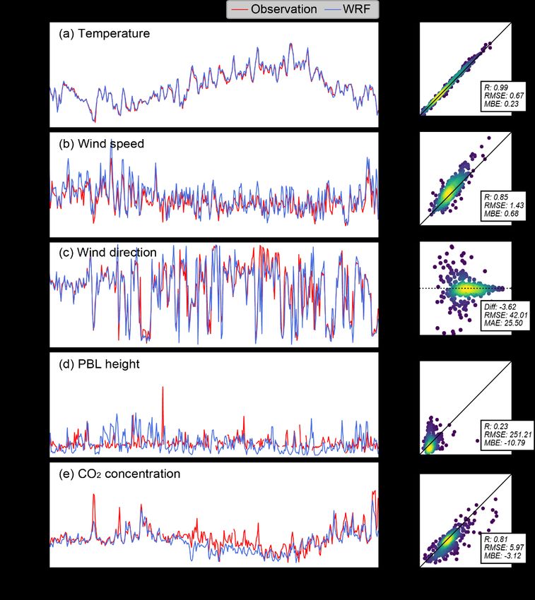
Figure S2: Time series of the daily nighttime mean (21-05 UTC) observed and BEP_MYJ modeled (a) temperature, (b) wind speed, (c)
     wind direction and (e) CO2 concentration at SAC100 station. (d) Time series of the daily nighttime mean (21-05 UTC) observed and
                                                    modeled PBL height at SIRTA station.
5
    Table S1. Meteorological conditions for several situations when large model-data misfits have been detected by the KNN algorithm.
               Date                                          Bulletin Climatique Météo-France*
     January 19-21, 2016        With the anticyclonic conditions, frosty fogs and stubborn low clouds were observed.
                                Temperatures dropped below normal with local snow. The wind was weak to moderate.
     April 12-13, 2016          Disturbances crossed the region on 9th, followed by a rain-unstable rise from 10th to 13th.
     August 27, 2016            The weather was under some unstable intermissions, e.g., stormy on 27 th and 28th, then a
                                few showers remained on 29th.
     October 25, 2016           With the gradual increase of pressure until 1035 hPa on 28 th, low clouds and fogs were
                                tenacious.
     …                          …
    * Accessible at: https://donneespubliques.meteofrance.fr/?fond=produit&id_produit=129&id_rubrique=29

                                                                                                                                        2
Figure S3: (left) Time series of the observed and MYJ_BEP modeled hourly CO2 concentration at SAC station from Jan 18th to 21st
2016. The grey shaded areas indicate the ranges of simulation results with five physical schemes used in this study (Table 1a in the
manuscript). The yellow vertical lines indicate the large model-observation misfits (outliers) detected by the K-nearest neighbors
5 (KNN) algorithm. (right) Distribution of the hourly CO 2 concentrations as a function of the wind speed for the year 2016.
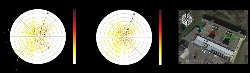
Figure S4: (a) Hourly CO and CO2 concentration measurements as a function of wind speed and direction at OVS station for the year
2016. (b) Image of the rooftop at OVS station with the CRDS CO & CO 2 sampling inlet in cyan and the building exhaust air system in
red and green.
10
We performed some further analyses and validations of this method to support the approach and the related statements
in the manuscript. These analyses definitely show that the outliers generally correspond to either:
1) the model’s inability under specific meteorological conditions.
After analyzing the dates of the identified outliers, we found clusters of outliers that occur as the result of weather
15 episodes with a duration of one-to-few days. Several cases were identified and described in Table S1. One sample case,
presented here, shows unfavorable meteorological conditions from Jan 18th to 21st 2016. During this 4-day period,
with a return of the winter anticyclonic conditions over the entire region, dense fog and weak winds were observed.
Stubborn low clouds kept temperatures chilly with little snow. Figure S3a shows the time series of the observed and
modeled (using MYJ_BEP) hourly CO2 concentration at SAC station. The grey shaded areas indicate the ranges of
20 model results with five physical parameterization schemes used in this study (Table 1a in the manuscript). The yellow
vertical lines indicate the large model-observation misfits (outliers) detected by the KNN algorithm. It can be seen that
for the certain hours that were tagged as outliers, the differences between observed and modeled CO2 concentrations
can be as large as 70 ppm. Meanwhile, the spread of the simulations of CO2 is much larger than during the days before
and after this period, leading to a higher mean bias error and root-mean square error of the ensemble mean. Figure S3b
25 shows the distribution of the hourly CO2 concentrations as a function of the wind speed for the year 2016. It clearly
illustrates that the detected outliers occurred more often in weak-wind conditions (< 2.5m/s) which are difficult to
reproduce by the model. From this example, we can say that KNN can detect outliers corresponding to conditions when
the model physics encounters limitations.
2) the specific measurement contaminations from local unresolved sources of CO2 emissions.
30 On the other hand, this KNN method was inspected for its ability to remove some CO2 spikes due to very local
influences or sampling contaminations, mainly under low wind speed conditions. We illustrate this phenomenon with
the example of the measurements of hourly CO and CO2 concentrations (CO being used to confirm the anthropogenic
origin of the spikes in the atmospheric concentration) at the OVS station in 2016. The CO and CO 2 hourly mole
3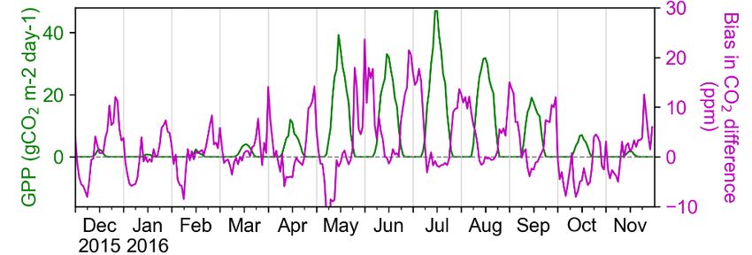
fractions, as well as their ratios, are plotted as a function of observed wind speed and direction (Figure S4a). The
     location of the CRDS CO & CO2 sampling inlet is on a building roof, where there is a building ventilation exhaust
     shown in Figure S4b. Figure S4a shows that the CO signal tends to be larger relative to that of CO2 with low winds (<
     4m/s) blowing from the east. This corresponds to the position of the building exhaust air system relative to that of the
 5   sampling inlet, and this is at odd with the North East position of the Paris urban area or of the main neighbor and large
     area sources relative to the OVS site. Further investigation shows that these CO spikes at OVS are mostly measured at
     night in winter, leading to a nighttime mean concentration even much larger than those two urban stations (JUS and
     CDS). We thus highly suspect that the measurements of CO and CO2 are contaminated by the exhaust air of the building
     under specific conditions (winter nighttime with light winds). Most of the dates corresponding to these CO and CO 2
10   spikes exactly coincide with the outliers at OVS that have been detected by the KNN algorithm shown in Figure 5 in
     the manuscript. From this example, we can say that KNN can detect outliers (in the data) corresponding to real physical
     local contaminations.
     Therefore, the KNN method, as shown above, can detect misfits between the observations and the models that would
     be misleading for the city scale inversions. But we also acknowledge the fact that removing data points simply based
15   on statistical analysis without identifying the outliers on a case-by-case basis may lead to a loss of data that are suitable
     for the city scale inversion. In practice, manual inspection is preferable for the identification of the cause of the error.
     However, this is not practical given a large amount of data at six in situ stations collected over one year as those
     analyzed in this study. It is also difficult to find a general outlier detection method fitting to any site, model and
     atmospheric transport conditions.
20

      Figure S5: Mean diurnal cycle of the modeled gross primary production (GPP) at SAC (green line, left scale), and the misfit between
        the modeled and observed CO2 horizontal differences between CDS and SAC (magenta line, right scale) for 12 calendar months.

25

                                                                                                                                            4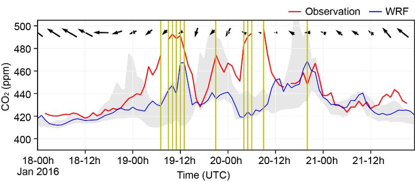
Figure S6: Daily nighttime mean (21-05 UTC) CO2 differences. (a) horizontal differences between CDS and COU; Vertical differences
    at TRN (c) between 5 m and 100 m AGL, and (c) between 50 m and 100 m AGL; Vertical differences at OPE (d) between 10 m and 120
5                                            m AGL, and (e) between 50 m and 120 m AGL.

                                                                                                                                   5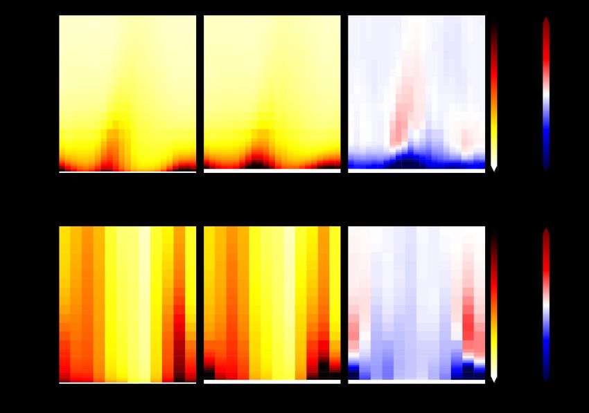
Figure S7: (a) Annual average of the vertical distributions of CO 2 concentrations at JUS station for 24 hours of the day for BEP, UCM
     and their differences; (b) Vertical distributions of CO 2 concentrations during afternoon (11-16 UTC) at JUS station for 12 calendar
                                                  months for BEP, UCM and their differences.
5

                                                                                                                                         6
You can also read