Synergy between Ocean Variables: Remotely Sensed Surface Temperature and Chlorophyll Concentration Coherence - MDPI
←
→
Page content transcription
If your browser does not render page correctly, please read the page content below
remote sensing
Letter
Synergy between Ocean Variables: Remotely Sensed
Surface Temperature and Chlorophyll
Concentration Coherence
Marta Umbert 1,2, * , Sebastien Guimbard 3 , Joaquim Ballabrera Poy 1,2           and Antonio Turiel 1,2
 1    Departament of Physical and Technological Oceanography, Institut de Ciències del Mar, CSIC,
      08003 Barcelona, Spain; joaquim@icm.csic.es (J.B.P.); turiel@icm.csic.es (A.T.)
 2    Barcelona Expert Center on Remote Sensing, CSIC-UPC, 08003 Barcelona, Spain
 3    Ocean Scope, Plouzané, 29280 Brest, France; sebastien.guimbard@ocean-scope.com
 *    Correspondence: mumbert@icm.csic.es

 Received: 27 February 2020; Accepted: 29 March 2020; Published: 3 April 2020

 Abstract: The similarity of mesoscale and submesoscale features observed in different ocean scalars
 indicates that they undergo some common non-linear processes. As a result of quasi-2D turbulence,
 complicated patterns of filaments, meanders, and eddies are recognized in remote sensing images.
 A data fusion method used to improve the quality of one ocean variable using another variable
 as a template is used here as an extrapolation technique to improve the coverage of daily Aqua
 MODIS Level-3 chlorophyll maps by using MODIS SST maps as a template. The local correspondence
 of SST and Chl-a multifractal singularities is granted due to the existence of a common cascade
 process which makes it possible to use SST data to infer Chl-a concentration where data are lacking.
 The quality of the inference of Level-4 Chl-a maps is assessed by simulating artificial clouds and
 comparing reconstructed and original data.

 Keywords: remote sensing; ocean color; data fusion; data merging; physical oceanography;
 singularity analysis

1. Introduction
      Global maps of Chl-a concentration at sea surfaces, similar to what happens with many other
remote sensing products, suffer from data gaps. This is especially true for high-spatial resolution (few
kilometers) daily maps, where orbital voids add to the data loss due to clouds, aerosols or sunglint.
For this kind of products, gap-filling and noise-reduction techniques are required to provide uniform
products suitable for environmental monitoring or the initialization of ecosystem models. To achieve
this goal, data interpolation and noise reduction are commonly performed using univariate methods
as, for example, [1]. Multivariate methods have also been applied to generate uniform products that
combine information from different sensors; examples of multivariate approaches include optimal
interpolation [2], empirical orthogonal functions [3,4], classification methods [5] and more recently
using data-diven methods as analog data assimilation [6,7]. The method discussed in this paper is
based on the empirical perception that fronts, eddies, and filaments are identifiable in the satellite
imagery of different ocean variables (sea level, ocean color, sea surface temperature, sea surface salinity)
and, sometimes, even in the raw radiance recorded by the satellites [8,9]. Remote sensing and drifter
data have shown that the statistical distribution of surface ocean fields has characteristics of a flow in
fully developed quasi-2D turbulence. Owing to the underlying turbulence of the ocean, the application
of a technique known as singularity analysis [10] allows to retrieving information about ocean currents
from images of any advected scalar.

Remote Sens. 2020, 12, 1153; doi:10.3390/rs12071153                      www.mdpi.com/journal/remotesensing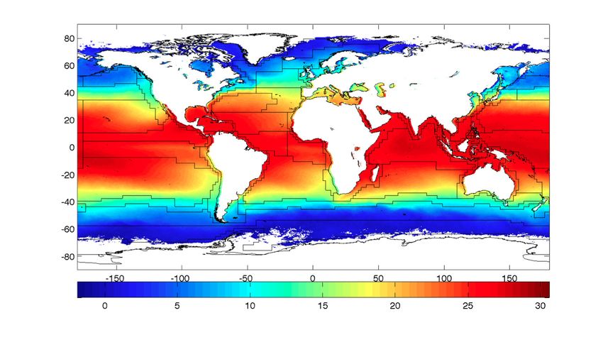
Remote Sens. 2020, 12, 1153                                                                        2 of 13

      The analysis of the spatial variability of pigment images found no difference between the
wavenumber spectra of SST and ocean color maps, leading to the conclusion that phytoplankton
cells in dynamic areas effectively behave as passive scalars [11,12]. In [13] it was shown that sea
surface temperature and chlorophyll maps have the same multifractal structure. This fact can be
interpreted as a consequence of the turbulent advection at the scales of observation and due to
the existence of a common cascade process [14]. The multifractal structure of any scalar can be
characterized through singularity analysis [15]. Singularity analysis is any technique capable of
calculating a map of the singularity exponents associated with a given scalar. A singularity exponent
is a non-dimensional number that characterizes the sharpness, or regularity, of the scalar around a
given point [10]. Nieves et al. [13] showed that the singularity exponents extracted from SST, Chl-a or
brightness temperature maps are very similar, a fact that was interpreted as an effect of the advection
term. Notice that the equivalence among singularity exponents does not require advection to be the
largest term in the equation of evolution. Advection is a non-linear term in the equation of evolution,
and thus it is at the origin of singularities.
      That the common singular structure of variables advected by the turbulent ocean has been
exploited to reduce the noise in SMOS sea surface salinity maps using data from auxiliary, high-quality
SST maps [16,17]. The same algorithm can be used not only to reduce noise but also to extrapolate
provided that the template is defined at the missing points. Although the theoretical foundation of the
data fusion method is relatively complex, its practical application is rather simple: a non-parametric,
weighted local linear regression between Chl-a and SST maps are calculated at each point, then the
regression parameters obtained at each point are applied to the value of SST at that point to infer a
new variable of Chl-a.
      The goal of this work is to assess the ability of a local linear regression approach to fill remote
sensing chlorophyll concentration data gaps. This local relation between SST and Chl-a can be
built from a single snapshot of both variables, so the implementation of the method is simple,
computationally fast, and no training set is required; moreover, the method is well fit to deal with
strong, rapid changes in the dynamics of the flow as far as it is always turbulent. Additionally,
the analysis of the auxiliary parameters of the fusion algorithm allows characterizing the modulation
of the seasonal correlation modulation between Chl-a and SST variables.

2. Satellite Data
     Two Aqua-MODIS ocean products from the NASA Aqua spacecraft are used in this study: Chl-a
concentration Level-3 daily product, and standard MODIS Aqua Level 3 SST Thermal IR Daily 4
km Nighttime, both at 4 km × 4 km grid [18]. Our dataset period goes from January to December
2006. The data were downloaded from the Ocean Color web portal, http://oceancolor.gsfc.nasa.gov/.
According to many studies, it is assumed that Chl-a follows a lognormal distribution [19] and so we
work with the logarithm of chlorophyll concentrations for ease of use (theoretically the singularity
exponents should not change if a monotonic function is applied to the data [10], but it is numerically
more stable to work with a dynamic range comprising fewer orders of magnitude).

3. Method

3.1. Singularity Analysis
     Singularity analysis is the key stone of the so-called Microcanonical Multifractal Formalism
(MMF) [10]; where the fluid is understood as a hierarchical arrangement of different fractal components,
each own with its own fractal dimension and characterized by a particular value of the singularity
exponent. Singularity exponents are related to the ocean circulation and thus they are not specific
to any particular scalar under study. In fact, it has been verified that with a good approximation
singularity lines coincide with the streamlines of the flow [20], confirming that singularity exponents
are characterized by the flow and not scalar-specific. The emergence of such a singular structure is the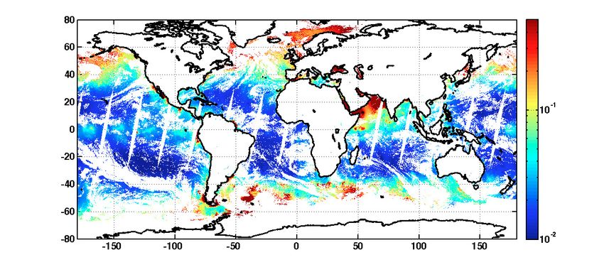
Remote Sens. 2020, 12, 1153                                                                             3 of 13

result of the advective forces acting on a quasi-2D turbulence regime, and can be thus observed for
scales ranging from kilometers to the planetary scale.
     The calculation of singularity exponents in a given noisy, discretized signal requires the use of an
appropriate interpolation scheme, the most usual one being wavelet projections. Let s be an arbitrary
2D scalar signal. It will be said that s has a singularity exponent h( x ) at the point x if, for any wavelet
function Ψ the following relation holds:

                                                                                x − x0

                                                                         1
                                                  Z
                              TΨ |∇s|( x, r ) ≡       dx 0 |∇s|( x 0 )      Ψ
                                                                         r2        r

                                                         = α ( x ) r h( x )   + o r h( x )                 (1)

where r stands for an arbitrary
                             scale
                                 parameter (normalized by the integral scale so it is dimensionless
and smaller than 1) and o r h( x) is a term that becomes negligible compared to r h( x) when r goes
to zero. The amplitude function α( x ) does not depend on the particular scale at which the wavelet
projection is calculated and has the same units as the gradient of the scalar.
     The left hand side, i.e., TΨ |∇s|( x, r ), is called the wavelet projection of the gradient modulus of s
over the wavelet Ψ, and represents a local zoom of variable size around the point x. What is important
in Equation (1) is the function h( x ), which is called the singularity exponent of the function s at the
point x. The singularity exponent is, by construction, a dimensionless measure of the regularity or
irregularity of the function s around the point x.

3.2. Fusion Method
      As discussed in Turiel et al. [10], ocean scalars as chlorophyll and temperature (denoted
respectively by c and θ) are multifractal in the microcanonical sense. This implies that a singularity
exponent can be assigned at each point and that they are arranged in a particular way, which in turn
implies that they are related to a property of the flow (its circulation) rather than to any specificity of
the associated scalar.
      Assuming that the singularity lines of Chl-a and SST coincide as it was shown in Nieves et al. [13],
it follows that their gradients must be related by a smooth 2 × 2 matrix ρ [17] :

                                              ∇c(~x ) = ρ(~x ) ∇θ (~x ),                                   (2)

    Although a large number of ρ(~x ) verifying Equation (2) exist, the indetermination is considerably
reduced by imposing that the matrix ρ(~x ) must be smooth: a non-smooth ρ(~x ) would be a source of
singularities, and hence the singularity lines of c and θ would differ. If we further assume that the
gradients of c and θ are aligned, then Equation (2) leads to:

                                            c(~x ) ≈ a(~x ) θ (~x ) + b(~x )                               (3)

with smooth functions a and b (i.e., they have small gradients as compared to those of c and θ).
     Let us now suppose that the function c is contaminated by some source of noise n, so in fact our
data sets consists of θ (~x ) (assumed noiseless) and c0 (~x ) = c(~x ) + n(~x ). We can construct a filtered
version of c, denoted by c f , as:
                                       c f (~x ) = â(~x ) θ (~x ) + b̂(~x )                               (4)

where â(~x ) and b̂(~x ) are estimates of the actual parameters a(~x ) and b(~x ) in Equation (3). These
estimates are obtained from the values of c0 and θ by performing scale-invariant linear regressions
weighted around each point. The weight of a specific point x 0 is defined as wx ( x 0 ) = | x − x 0 |−2 .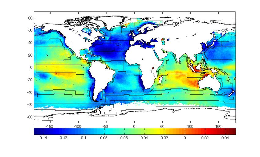
Remote Sens. 2020, 12, 1153                                                                           4 of 13

      The total weight of a point ~x, N (~x ), is defined as follows:

                                                                             1
                                          N (~x ) ≡      ∑0          |~x 0   − ~x |2
                                                                                                         (5)
                                                      ~x 6=~x ∈sea

     The weighted regression uses all available data of each field, using the function N (~x ) that decay
as a power-law with the distance (Equation (5)); thus it is scale-invariant, as it does not introduce any
preferred scale [16,17].
     With â(~x ) and b̂(~x ), an estimation of the chlorophyll c f may be obtained applying Equation (4) as
soon as the value of θ at that location ~x is available. This algorithm was shown in Umbert et al. [17] to
lead to a large increase in the quality of SMOS SSS maps using OSTIA SST maps as a template; besides,
the method leads to significant restoration of the structure of singularity exponents.

4. Results

4.1. Scalar Synergy
     Figure 1 shows examples of daily maps of MODIS Chl-a concentration (top panel) and SST
(middle panel) in 1 January 2006. The values of Chl-a are derived from measurements in the visible
part of the spectrum, which may be affected by artifacts like aerosols, sun glint and high turbidity
of the water. Several flags are introduced to characterize Chl-a data quality and a result, maps of
Chl-a usually suffer from a larger incompleteness than those of SST, which are derived from infrared
measurements in the 4 µm range. An example of the application of the fusion algorithm in the global
ocean for 1 January 2006 is shown in the bottom panel of Figure 1. As stated before, the algorithm
allows estimating the local Chl-a-SST regression by taking into account all possible couples of data
(SST,Chl-a) weighted using function N (~x ) in Equation (5). Fused Chl-a maps integrate the relation
between structures present in the SST and Chl-a specific structures. In fused daily products we
recognize some expected Chl-a global patterns, near the ocean surface, where availability of sunlight is
not limiting, phytoplankton growth depends on temperature and nutrient levels. High chlorophyll
concentrations are found in nutrient-rich, cold polar waters and where ocean currents cause upwelling,
which brings nutrient-rich deep-cold water to the surface.
     We will focus in the region of the Gulf of California, a narrow sea between mainland Mexico
and the Baja California peninsula, where high primary productivity levels are found as a result of
an efficient nutrient transport of waters from under a shallow pycnocline into the euphotic zone [21].
Figure 2 shows the input variables of our algorithm (top panel: Chl-a, middle panel: SST) and the
output fused Chl-a (bottom panel). The corresponding singularity exponents are shown in the right
column. Rich singularity structures can be recognized in the original chlorophyll concentration maps
associated with the fronts mainly caused by the horizontal transport from high primary production
areas onto less productive ones. The SST field exhibits also the richness of patterns associated with
the circulation in that area. Where both images are not affected by data gaps, the singularity structure
(although not the magnitude) is similar between them. Places where the correspondence of both
singularity images fails may identify places at which intrinsic dynamics of the variable competes with
flow advection.
     Once the data fusion is applied, the L4 Chl-a is extrapolated to all the pixels where SST was
available. The structure of Chl-a is well represented (compared to the original image), although a
smoothing of the original variable degrades the dynamic range of the variable. The singularity
exponents of the fused Chl-a data reveal that most of the structures present in the SST map are
re-integrated in the chlorophyll map at the same time that Chl-a specific magnitude and structures are
maintained; for instance, the strong gradient associated with the biological activity present in the Gulf
of California, appear delineated in the fused Chl-a. This implies that the fusion algorithm can partially
integrate SST structures without destroying Chl-a ones.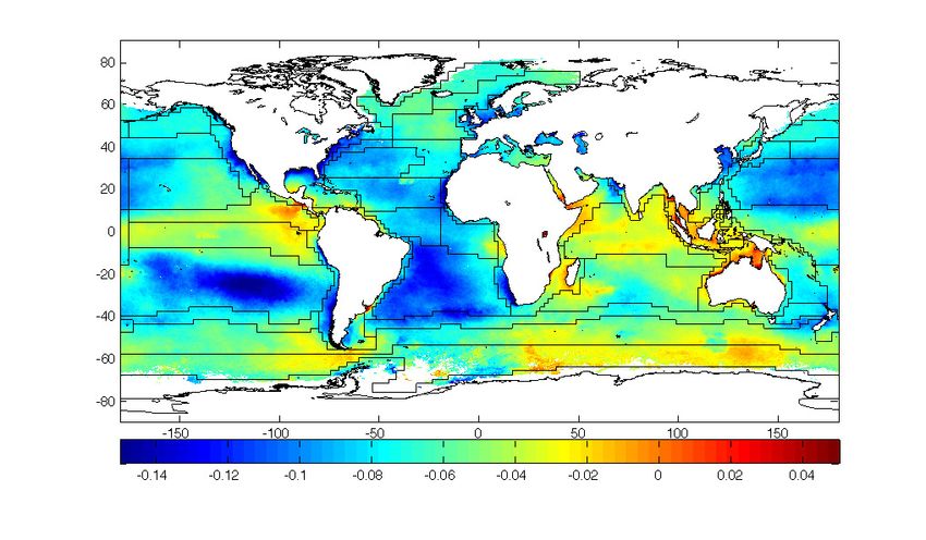
Remote Sens. 2020, 12, 1153                                                                         5 of 13

      Figure 1. (top panel) MODIS Aqua Level 3 Chl-a (mg/m3 ), (middle panel) MODIS Aqua Level 3 SST
      (◦ C) and (bottom panel) Level 4 Chl-a concentration (mg/m3 ) extended to the areas where MODIS
      SST was available, for 1 January 2006.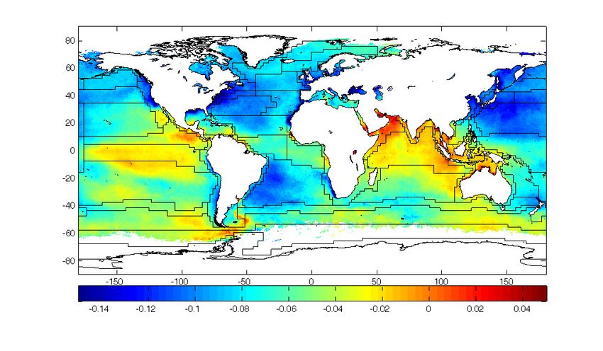
Remote Sens. 2020, 12, 1153                                                                               6 of 13

      Figure 2. (top row) MODIS Chl-a (mg/m3 ), (middle row) MODIS SST (◦ C) and (bottom row) fused
      Chl-a (mg/m3 ), for 1 January 2006 (left column) and associated singularity exponents (right column).

4.2. Interpretation of Auxiliary Parameters
     As shown in Equation (4), the functions â(~x ) and b̂(~x ) provide information about the local
functional dependence between SST and Chl-a. The local slope, â(~x ), will be negative at those places
where SST decreases as Chl-a increases in the neighborhood, and the converse. Considering that cold
waters tend to have more nutrients than warm waters, phytoplankton is more abundant where surface
waters are cold. So, as we move from one given point to another with colder water, Chl-a would
usually increase and thus the slope â(~x ) will be negative. However, the relationship changes from
point to point and it should be expected to change from one image to the next one. Figure 3 shows the
seasonal average of the slope and intercept (considering winter as January-February-March, spring as
April-May-June, summer as July-August-Septemebr and fall as October-November-December).
     The coherent patterns of the auxiliary parameters of the method delineate areas with different
relation between Chl-a and SST. In the same spirit, Longhurst [22] introduced the concept of
ocean biogeochemical provinces, characterized by their particular physical and biological behavior.
Longhurst definition is based on the mixed layer depth lying close to the ocean-atmosphere interface.
Specific provinces have common characteristics and can generally be classified as four general biomes:
the coastal, polar, westerly and trade winds biomes. A visual comparison between local functions of
the fusion method and the Longhurst definition is shown in Figure 3.
     As expected, negative slopes are present in the upwelling areas associated with the easternmost
currents of the great anticyclonic gyres, corresponding to the Benguela and Canary currents in the
Atlantic Ocean and the Peru and California currents in the Pacific Ocean. Notice that this negative
slope is present all year long. These oceanic areas, as well as the upwelling zones and continental
margins, are rich in Chl-a as a result of the proximity to areas where the resurgence of nutrients take
place and the local circulation is favorable to nutrient accumulation. A band of cool, chlorophyll-rich
water is also apparent all along the equator; the strongest signal at the Atlantic Ocean and the open
waters of the Pacific Ocean also leads to negative values of the local intercept b̂(~x ).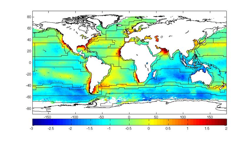
Remote Sens. 2020, 12, 1153 7 of 13
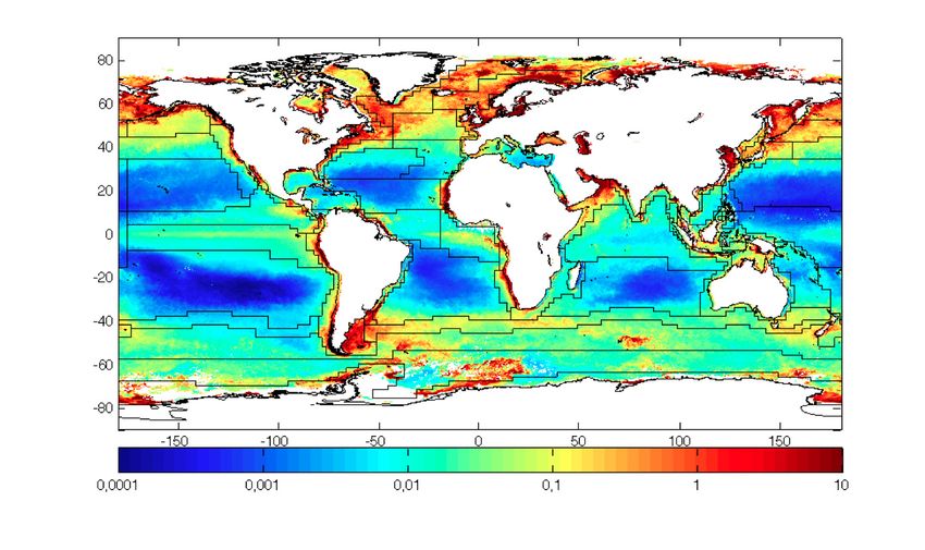
Figure 3. (left column) Seasonal mean local slope estimation â( x ) for spring, summer, fall and winter.
(right column) Local intercept estimation b̂( x ) for spring, summer, fall and winter. These are the mean
estimations used in the derivation of the fused maps as the one presented in Figure 1. (bottom row)
Chl-a mean concentration for year 2006 and SST mean for the same year.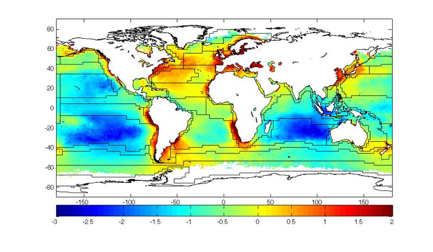
Remote Sens. 2020, 12, 1153                                                                        8 of 13

     Negative values of â(~x ) are also found in areas where Chl-a concentration decreases as SST
increases; this situation, which is typically found in the (oligotrophic) subtropical gyres, intensifies
in the Atlantic Ocean during the northern hemisphere winter and spring. The Pacific Ocean exhibits
an intensified negative pattern in the Northern subtropical gyre during boreal spring and a negative
pattern in the southern hemisphere during austral spring. In both cases, such intensification in the
oligotrophic subtropical gyres is driven by the seasonal cycle of sea surface temperature.
     Subpolar gyres are also characterized by high Chl-a concentrations linked to nutrient accumulation
during winter, when the mixing layer reaches the deep ocean followed by the stratification of the
water column during spring. During the dark winter months, the local slope between SST and Chl-a is
positive. However, when sunlight returns and nutrients are trapped near the surface during spring
and summer, the phytoplankton flourishes in high concentration, seen as negative values of â(~x ).
     The local regression coefficient (not shown) has small values along the Equatorial Pacific, and in
the Southern and Indian Ocean indicating that horizontal advection of Chl-a cannot be locally explained
by SST variability in these regions only. Therefore, either additional variables should be taken into
account, or a more sophisticated relation between Chl-a and SST should be used. For example, in ocean
regions of High Nutrient Low Chlorophyll (HNLC) as the equatorial Pacific and the Southern Ocean,
low Chl-a concentrations are due to a stoichiometric imbalance of iron which have no link to SST.
Another possible cause for the low values of the local regression coefficient in some regions is the lack
of enough points to provide a quality reconstruction. For instance, 85% of the data points are missing
in the Equatorial Pacific due to the large cloudiness.

4.3. Validation of Reconstruction
      To assess the quality of the extrapolation resulting from our data fusion method, we validate
it by analyzing 5 different regions (as shown in Figure 4); each region has at least an area of 8 × 8
degrees (200 × 200 pixels). For each of these areas a mask representing a cloud structure (of the typical
size and shape found in chlorophyll images) is defined (the clouds are generated using a real MODIS
SST 9-km daily image of 1 January 2006, and are kept fixed in time). Those masks have a surface of
about 30% of the region on which they will be applied. To assess the quality of the fusion algorithm,
we proceed in three steps. In the first step, points lying in the masked area of a daily Chl-a map are
removed (notice that there will be additional missing points in the Chl-a map because of the gaps in
the original remote sensing product; for instance, in the EP area (Figure 4) the average percentage of
missing points is 85%). In the second step, the fusion algorithm is applied to the masked Chl-a map
using the corresponding daily SST map as a template, extrapolating to the missing values. Finally,
the extrapolated values are compared to the available original ones on the masked area for each image
during the entire year 2006 (365 daily images). We require a minimum of 5% of original Chl-a values
existed inside the masked area to perform the cross validation. This strategy allows comparing the
original Chl-a and the retrieved one at the available masked points, and therefore the extrapolation
ability of the fusion method.
      The performance of the algorithm is studied in different Chl-a regimes: oligotrophic regions
(Central Atlantic, CA and Pacific in front of California, CL) and eutrophic regions in higher latitudes
(North Atlantic, NA), coastal upwelling areas (Benguela upwelling, BG) and the Equator (Equatorial
Pacific, EP). NA region is defined by [19.61◦ W–9.19◦ W; 51.65◦ N–57.91◦ N] and 22% of the area is
masked, EP region is defined by [142.54◦ W–130.04◦ W; 5.02◦ S–0.40◦ N] (29% of the area is masked),
CL region is defined by [125.87◦ W–117.53◦ W; 22.48◦ N–30.82◦ N] (31% of the area is masked), BG region
is defined by [9.56◦ E–17.90◦ E; 27.53◦ S–19.19◦ S] (35% of the area is masked) and CA is defined by
[40.44◦ W–30.03◦ W; 22.48◦ N–30.82◦ N] with a 34% of the area being masked.
      Examples of one daily image validation are shown in Figure 4 for each region. A quantitative
measure of the quality of the reconstruction of the chlorophyll is given in terms of four parameters:
the root mean square (rms), bias (mean) and standard deviation (std) of the reconstructed error and
the correlation coefficient (r) between the masked and reconstructed values. In the case of the central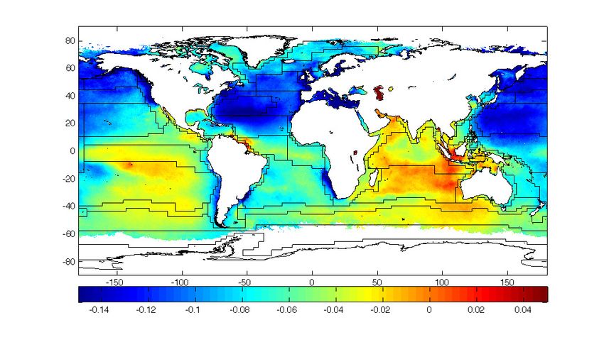
Remote Sens. 2020, 12, 1153                                                                                           9 of 13

Atlantic and California regions, the concentration of chlorophyll is smaller, followed by the values
found in the North Atlantic, the Equatorial Pacific and the Benguela upwelling where highest values
of Chl-a concentration are found. Correlations coefficients between L4 and original Chl-a decrease for
the regions where lower pigment concentrations are found. Better statistics are associated to areas of
high primary production.
      The validation for the entire year 2006 is summarized in Table 1; the mean seasonal values for each
one of the statistical parameters and clouds are included. Our data fusion method succeeds in filling
gaps with mean annual correlation coefficients ranging from 0.58 to 0.81 for the studied period and
artificial clouds. Oligotrophic regions (North Atlantic and California) have mean regression coefficients
which are significantly lower than the mean correlation coefficients values for the equatorial Pacific,
the North Atlantic and the Benguela upwelling regions respectively. The smaller performance in
oligotrophic regions is probably due to the small horizontal gradients of Chl-a there together with
a larger signal-to-noise ratio. However, the absolute error of the reconstruction is always moderate.
A slightly mean positive bias is systematically found, meaning that the L4 estimates are smaller than
the original Chl-a values, probably due to the smoothing generated by the weighting function used in
the fusion algorithm [16].
      The seasonal segregation of validation results highlights a worse performance during the
January-February-March period, with mean correlation coefficients ranging from 0.15 to 0.47 (Central
Atlantic and Benguela upwelling, respectively). During the rest of seasons, the validation results
greatly improve with correlation coefficients ranging from 0.67 to 0.94 in spring (AMJ), from 0.77 to
0.94 in summer (JAS) and from 0.74 to 0.94 in fall season (OND). In the winter season, the strengthening
of winds and deepening of the mixed layer in mid and high latitudes create a large supply of nutrients
from the deep ocean to the surface, which will be available for phytoplankton to proliferate in the
following seasons. In equatorial and coastal upwelling regions (Equatorial Pacific and Benguela,
respectively), the upwelling intensity also varies seasonally depending on wind strength and direction
and the vertical structure of the water column. Under these circumstances, nutrient availability, vertical
mixing and the depth of the mixed layer play crucial roles in the distribution of Chl-a, which could not
be only explained by horizontal advection and the distribution of surface temperature.
      The power density spectra (PDS) is computed as in [23] inside the boxes shown in in Figure 5
(top) for each daily file and then the median for the entire period 2006 is calculated. The spatial
spectral analysis of MODIS Chl-a, MODIS L3 SST and Level 4 Chl-a products under the SPURS and
STP regions (red and green boxes in Figure 5 (top)) shows that the actual spatial resolution of MODIS
Chl-a and MODIS L3 SST is about 10 km and, and 15 km for the L4 Chl-a product (Figure 5 (bottom)).
The intermittent character of MODIS Chl-a and the lower resolution of L4 Chl-a explain the vertical
shift between their PDS.

       Table 1. Mean seasonal results of daily reconstruction validation under artificial clouds for year 2006.

                       R                           ST D                        BI AS                       RMS
         JFM    AMJ        JAS    OND    JFM    AMJ    JAS    OND    JFM    AMJ    JAS    OND    JFM    AMJ    JAS    OND
  CA     0.15   0.67       0.77   0.74   0.20   0.07   0.08   0.06   0.70   0.04   0.03   0.02   0.73   0.08   0.09   0.06
  BG     0.47   0.93       0.91   0.93   0.35   0.14   0.13   0.11   0.27   0.03   0.02   0.02   0.47   0.15   0.13   0.12
  CL     0.19   0.89       0.80   0.88   0.22   0.04   0.04   0.04   0.72   0.02   0.03   0.03   0.75   0.05   0.05   0.06
  EP     0.25   0.94       0.94   0.94   0.17   0.04   0.03   0.03   0.42   0.01   0.02   0.01   0.46   0.04   0.04   0.03
  NA     0.33   0.88       0.91   0.86   0.16   0.09   0.10   0.07   0.47   0.02   0.01   0.01   0.50   0.10   0.10   0.07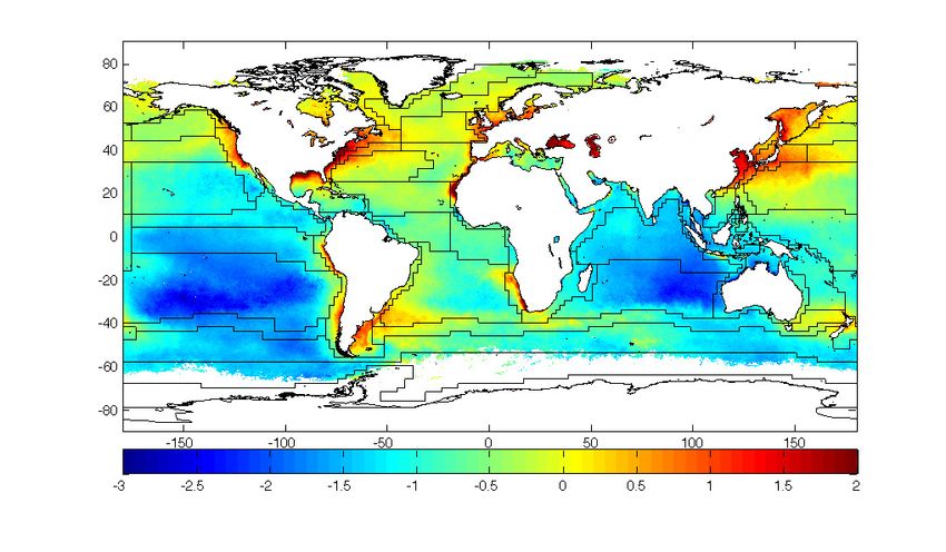
Remote Sens. 2020, 12, 1153 10 of 13
Central Atlantic (day 95) chlorophyll
x=y
R = 0.70 linear regression
MEAN = -0.02
STD = 0.05
RMS = 0.06
Level4 CHL mg.m - 3
10-1
10-2
10-2 10-1
MODIS-Aqua CHL mg.m - 3
102
Benguela (day 159) chlorophyll California (day 90) chlorophyll
x=y x=y
R = 0.95 linear regression R = 0.94 linear regression
MEAN = 0.03 MEAN = -0.02
STD = 0.15 STD = 0.04
RMS = 0.15 RMS = 0.05
101
Level4 CHL mg.m - 3
Level4 CHL mg.m - 3
10-1
100
10-1
10-2 -2 10-2 -2
10 10-1 100 101 102 10 10-1
MODIS-Aqua CHL mg.m - 3 MODIS-Aqua CHL mg.m - 3
100 101
Equatorial Pacific (day 193) chlorophyll North Atlantic (day 193) chlorophyll
x=y x=y
R = 0.97 linear regression R = 0.93 linear regression
MEAN = 0.01 MEAN = -0.02
STD = 0.04 STD = 0.11
RMS = 0.04 RMS = 0.11
Level4 CHL mg.m - 3
Level4 CHL mg.m - 3
100
10-1 -1 10-1 -1
10 100 10 100 101
MODIS-Aqua CHL mg.m - 3 MODIS-Aqua CHL mg.m - 3
Figure 4. Artificial clouds generated for validation purposes in the Central Atlantic (CA), Benguela
upwelling (BG), California Pacific (CL), Equatorial Pacific (EP) and North Atlantic (NA) (top left panel).
Validation of reconstruction under artificial clouds for MODIS Chl-a concentration. For CA region day
95, BG region day 159, CL day 90, EP day 193, and NA day 193 of year 2006.Remote Sens. 2020, 12, 1153 11 of 13
Figure 5. (top) Areas for power density spectra (PDS) computation: Red box represent SPURS region
(22◦ –28◦ N and 28◦ –60◦ W) and green box represent STP region (27◦ –33◦ S and 106◦ –170◦ W). (bottom)
Median of PDS for the year 2006 of MODIS L3 SST, MODIS Chl-a, and Level 4 Chl-a for the SPURS
region (left) and the STP region (right).
5. Discussion and Conclusions
Satellite missions that measure chlorophyll concentration offer limited coverage due to orbital
gaps, the presence of clouds and aerosols, sun glint, poor retrieval of the geophysical variables, etc.
Combining data from several satellites can considerably increase the spatial coverage of daily maps.
In this paper, we have used a method to merge the information coming from two different ocean
scalars that share common multifractal characteristics. One of the two scalars, denoted as template,
is assumed to have higher spatial coverage and signal-to-noise ratios than the other one, denoted
as signal. The application presented here uses MODIS SST as template and MODIS Chl-a as signal.
The template is used to extrapolate the signal by estimating local linear regression coefficients between
Chl-a and SST, then applying them to the template to restore the signal.
The regression coefficients of the data fusion method exhibit geographical patterns that contain
information about the relation between Chl-a and SST. The linear approximation, based on the
hypothesis that the gradients of the regression coefficients are negligible as compared with the gradients
of the variables Chl-a and SST, is less accurate on equatorial Pacific, Indian oceans, and during
the winter season. In all these cases the present scheme needs to be extended. Besides, auxiliary
environmental information, such as surface winds, mixed layer depth or nutrient concentration must
be taken into account to fully understand the Chl-a behavior.Remote Sens. 2020, 12, 1153 12 of 13
By exploiting the synergy between Chl-a and SST, it has been possible to increase the daily spatial
coverage of MODIS Chl-a. The extrapolated fields have proved to be consistent with the observed
ocean structures. A cross validation of the methodology, which consisted on create artificial gaps, apply
the methodology and compare to the original Chl-a data, indicates correlation coefficients ranging
from 0.67 to 0.94, except in winter season, when the correlation coefficients range from 0.15 to 0.47.
In conclusion, we have demonstrated the efficiency of blending SST and Chl-a to improve spatial
coverage of chlorophyll products and to study the relation between ocean scalars. The resulting
information can help to further characterize the spatio-temporal correlation between SST and Chl-a,
and the temporal variation and long-term evolution of the biogeochemical provinces.
Author Contributions: Conceptualization, A.T. and M.U.; methodology, A.T. and M.U.; software, M.U., S.G. and
J.B.P.; validation, M.U., S.G. and J.B.P.; writing—original draft preparation, M.U.; writing—review and editing,
M.U., S.G., J.B.P. and A.T.; visualization, M.U., S.G. and J.B.P.; supervision, A.T. and J.B.P.; funding acquisition,
A.T. and M.U. All authors have read and agreed to the published version of the manuscript.
Funding: M. Umbert is funded by the European Union’s Horizon 2020 research and innovation programme under
the Marie Skłodowska-Curie Individual Fellowship Career Restart Panel (MSCA-IF-EF-CAR Number 840374).
Acknowledgments: The authors acknowledge Ocean Color service website for making publicly available their
MODIS-Aqua data at http://oceancolor.gsfc.nasa.gov/. We acknowledge the insightful reviews, comments and
suggestions by anonymous reviewers that helped improve the content and readability of the manuscript.
Conflicts of Interest: The authors declare no conflict of interest.
References
1. Smith, T.M.; Reynolds, R.W. Improved extended reconstruction of sst (1854–1997). J. Clim. 2004, 17, 2466–2477.
[CrossRef]
2. Buongiorno, B. A novel approach for the high-resolution interpolation of in situ sea surface salinity. J. Atmos.
Ocean. Technol. 2012, 29, 867–879.
3. Alvera-Azcarate; Barth, A.J.; Weisberg, R. Multivariate reconstruction of missing data in sea surface
temperature, chlorophyll and wind satellite fields. J. Geophys. Res. 2007, doi:10.1029/2006JC003660.
[CrossRef]
4. Sirjacobs, D.A.; Alvera-Azcarate, A.; Barth, G.; Lacroix, Y.; Park, B.; Nechad, K.; Ruddick, J.-M.B. Cloud
filling of ocean colour and sea surface temperature remote sensing products over the southern north sea by
the data interpolating empirical orthogonal functions methodology. J. Sea Res. 2011, 65, 114–130. [CrossRef]
5. Jouini Lévy, M.M.; Crépon, M.; Thiria, S. Reconstruction of satellite chlorophyll images under heavy cloud
coverage using a neural classification method. Remote. Sens. Environ. 2013, 131, 232. [CrossRef]
6. Fablet, R.; Huynh Viet, P.; Lguensat, R.; Horrein, P.H.; Chapron, B. Spatio-Temporal Interpolation of Cloudy
SST Fields Using Conditional Analog Data Assimilation. Remote. Sens. 2018, 10, 2310. [CrossRef]
7. Lguensat, R.; Teo, P.; Ailliot, P.; Pulido, M.; Fablet, R. The analog data assimilation. Mon. Weather Rev.
2017, 145, 4093–4107. [CrossRef]
8. Crocke, E.R.W.; Matthews, D.; Baldwin, D. Computing ocean surface currents from infrared and ocean color
imagery. IEEE Trans. Geosci. Remote Sens. 2007, 45, 435–447. [CrossRef]
9. Isern-Fontanet; Turiel, J.A.; Garcia-Ladona, E.; Font, J. Microcanonical multifractal formalism: Application
to the estimation of ocean surface velocities. J. Geophys. Res. 2007, 112, C05024.10.1029/2006JC003878.
[CrossRef]
10. Turiel, A.H.; Pérez-Vicente, C. Microcanonical multifractal formalism: A geometrical approach to multifractal
systems. Part I: Singularity analysis. J. Phys. 2008, 41, 015501.10.1088/1751-8113/41/1/015501. [CrossRef]
11. Denman, K.L.; Abbott, M.A. Time scales of pattern evolution from cross-spectrum analysis of advanced very
high resolution radiometer and coastal zone color scanner imagery. J. Geophys. Res. 1994, 99, 7433–7442.
[CrossRef]
12. Doney, S.C.; Glover, D.M.; McCue, S.J.; Fuentes, M. Mesoscale variability of SeaWiFS satellite Ocean Color:
Global Patterns and spatial scales. J. Geophys. Res. 2003, 108, 6.1–6.15. [CrossRef]
13. Nieves, V.C.; Llebot, A.; Turiel, J.; Solé, E.; García-Ladona, M.; Estrada; Blasco, D. Common turbulent
signature in sea surface temperature and chlorophyll maps. Geophys. Res. Lett. 2007, 34, L23602. [CrossRef]Remote Sens. 2020, 12, 1153 13 of 13
14. Frisch, U. Turbulence: The Legacy of A.N. Kolmogorov; Cambridge University Press: Cambridge, MA, USA, 1995.
15. Turiel, A.; Parga, N. The multi-fractal structure of contrast changes innatural images: From sharp edges to
textures. Neural Comput. 2000, 12, 763–793. [CrossRef] [PubMed]
16. Olmedo, E.J.; Martínez, M.; Umbert, N.; Hoareau, M.; Portabella, J.; Ballabrera-Poy, A. Improving time and
space resolution of smos salinity maps using multifractal fusion. Remote. Sens. Environ. 2016, 180, 246–263.
[CrossRef]
17. Umbert, M.; Hoareau, N.; Turiel, A.; Ballabrera-Poy, J. New blending algorithm to synergize ocean
variables: The case of SMOS sea surface salinity maps. Remote. Sens. Environ. 2014, 146,
172–187.10.1016/j.rse.2013.09.018. [CrossRef]
18. Brown; O; Minnett, P.J. Modis Infrared Sea Surface Temperature Algorithm Algorithm Theoretical Basis
Document. Version 2.0. Available online: https://modis.gsfc.nasa.gov/data/atbd/atbd_mod25.pdf
(accessed on 2 April 2020).
19. Campbell, J.W. The lognormal distribution as a model for bio-optical variability in the sea. J. Geophys. Res.
1995, 100, 237–254. [CrossRef]
20. Turiel, A.; Nieves, V.; García-Ladona, E.; Rio, M.H.; Larnicol, G. The multifractal structure of satellite
temperature images can be used to obtain global maps of ocean currents. Ocean. Sci. 2009, 5, 447–460.
[CrossRef]
21. Valdez-Holguin, J.E.; Lara-Lara, J.R. Primary productivity in the gulf of california effects of el 350 niño
1982-1983 event. Cienc. Mar. 1987, 13, 34–50. [CrossRef]
22. Longhurst, A.R. Ecological Geography of the Sea; Academic Press: Cambridge, MA, USA, 1998.
23. Hoareau, N.; Turiel, A.; Portabella, M.; Ballabrera-Poy, J.; Vogelzang, J. Singularity power spectra: A method
to assess geophysical consistency of gridded products—application to sea-surface salinity remote sensing
maps. IEEE Trans. Geosci. Remote. Sens. 2018, 56, 5525–5536. [CrossRef]
c 2020 by the authors. Licensee MDPI, Basel, Switzerland. This article is an open access
article distributed under the terms and conditions of the Creative Commons Attribution
(CC BY) license (http://creativecommons.org/licenses/by/4.0/).You can also read