Teaching resource: 1970 British Cohort Study Malaise Inventory - Introducing quantitative analysis using SPSS

Teaching resource: 1970 British Cohort
Study Malaise Inventory
Introducing quantitative analysis using SPSS

Copyright © 2021 University of Essex.
Created by UK Data Archive, UK Data Service.

Introduction
The Centre for Longitudinal Studies (CLS) - funded under the ESRC Researcher
Development Initiative - has created a set of teaching datasets and associated resources
based on the National Child Development Study (NCDS) and the 1970 British Cohort Study
(BCS70).

The UK Data Service has converted part of the resource, exercises on measuring signs of
psychological distress or depression in teenagers and adults using the BCS70, into an
online step-by-step guide which can be used in conjunction with the data.

The guide includes information on how to access the data, an introduction to the
established set of survey questions that measures psychological distress - the Malaise
Inventory - and a number of data analysis exercises using SPSS.

Purpose of this resource

The data and resources are aimed for use with undergraduates and postgraduates and are
designed to be used with SPSS (though the data are also made available in Stata and tab-
delimited formats).

The resource can serve both as an introduction to the Malaise Inventory - an established
scale to measure signs of psychological distress - and as an introduction to quantitative
analysis using SPSS.

The techniques covered range from introductory descriptive statistics to multiple and logistic
regression. The resource will probably work best where the students have some familiarity
with the software package but not the techniques covered, or vice versa. However, no prior
knowledge is assumed.

Accessing the data
The dataset to accompany this teaching resource needs to be downloaded from SN 5805
British Cohort Studies Teaching Dataset for Higher Education, 1958-2000.

This can be obtained by UK Data Service registered users and is subject to UK Access
Management Federation (UKAMF) authentication. Further information on registration and
login can be found on the Registration and FAQs help page.

Teachers wishing to share the data with students should follow the guidance on the
Accessing and sharing data for teaching page.

                                                 Teaching resource: 1970 BSC Malaise Inventory | 4 |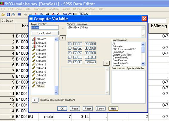

Introduction to the data
The dataset which will be explored as part of this exercise is b034malaise.sav, a subset of
data from the BCS70.

This longitudinal dataset includes information allowing you to look at the relationship
between socio-economic circumstances in childhood and mental well-being in adulthood
over time. The file contains 135 variables, representing information collected from cohort
members’ birth in 1970 up to 2004, when they had reached age 34.

Data collected:

   •   from birth are provided by the cohort members’ mothers
   •   at age 5, age 10 and age 16 were collected from the mother (or father)
   •   at age 26, 30 and 34 the cohort member themselves provided the information

There are:

   •   18,732 cohort members in the dataset
   •   9,740 (52 per cent) are men
   •   8,984 (48 per cent) are women
   •   8 did not have a sex recorded at their premature birth

The number of cohort members answering at least one Malaise question were:

   •   5,539 at age 16
   •   8,968 at age 26
   •   11,112 at age 30
   •   9,598 at age 34

   •   6,360 answered at least one Malaise question at age 26, 30 and 34
   •   2,970 answered at least one Malaise question at age 16, 26, 30 and 34.

To enable the information included here to be cross-referenced with the original
questionnaire documentation, original variable names are included in the variable label.

This file can also be merged with the b016mothermalaise.sav file to look at the relationship
between a mother and her child’s mental well-being.

Background to the Malaise Inventory
At various ages from teenager to adulthood, BCS70 cohort members have completed the
Malaise Inventory (Rutter et al., 1970) - a set of self-completion questions which combine to

                                                Teaching resource: 1970 BSC Malaise Inventory | 5 |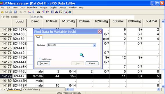

measure levels of psychological distress, or depression. The 24 ‘yes-no’ items of the
inventory cover emotional disturbance and associated physical symptoms. When
administered in its standard format, scores range from 0 to 24.

The Malaise Inventory was itself developed from the Cornell Medical Index Health
Questionnaire (CMI) which is comprised of 195 self-completion questions (Brodman et al.,
1949, 1952). Fourteen of the 24 questions are taken directly from the CMI (Rutter et al.,
1970). Individuals responding ‘yes’ to eight or more of the 24 items are considered to be at
risk of depression (Rodgers et al., 1999).

The internal consistency of the scale has been shown to be acceptable and validity of the
inventory shown to hold in different socio-economic groups (Rodgers et al., 1999).

The scale has been used in both general population studies (McGee, Williams and Silva,
1986; Rutter and Madge, 1976; Rodgers et al., 1999) and in investigations of high-risk
groups (Grant, Nolan and Ellis, 1990).

Rutter himself affirms that 'the inventory differentiates moderately well between individuals
with and without psychiatric disorder' (Rutter et al., 1970, p160).

The individual questions and the ages they have been asked in the two cohorts are detailed
in the next section.

Questions
In the BCS70, all 24 'yes-no' questions were asked in the standard way at age 26 and age
30 but at age 34, just 9 of the 24 questions were asked (again in the standard 'yes-no'
format).

However, when BCS70 cohort members were aged 16 they were asked 22 of the 24
questions and a three answer category approach was adopted:

   •   0='rarely/never'
   •   1='some of the time'
   •   2='most of the time'

When questions are asked in the standard format:

   •   1 point is awarded for every 'yes' response
   •   0 points for every 'no' response.

An overall Malaise score for a cohort member is the sum across the individual variables,
yielding a minimum score of 0 and a maximum of 24.

                                                 Teaching resource: 1970 BSC Malaise Inventory | 6 |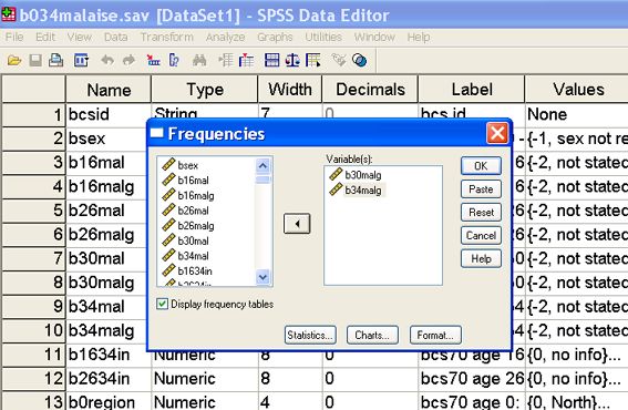

A score of 8 or higher is considered to be a sign that the cohort member is experiencing
symptoms associated with depression.

When only 9 questions were included, a score of 4 or higher is considered to be a sign that
the cohort member is experiencing symptoms associated with depression.

The overall Malaise score range for BCS70 cohort members at age 16 (when a three
answer category approach was adopted) has a minimum of 0 and a maximum of 44. A
score of 15 or higher is considered to be a sign that the cohort member is experiencing
symptoms associated with depression.

Table 1: Age individual Malaise questions were asked in BCS70

Question                                          Age 16    Age 26     Age 30    Age 34
1. Do you often have backache?                    yes       yes        yes       no
2. Do you feel tired most of the time?            yes       yes        yes       yes
3. Do you often feel depressed?                   yes       yes        yes       yes
4. Do you often have bad headaches?               yes       yes        yes       no
5. Do you often get worried about things?         yes       yes        yes       yes
6. Do you usually have great difficulty in falling
                                                   yes      yes        yes       no
or staying asleep?
7. Do you usually wake unnecessarily early in
                                              yes           yes        yes       no
the morning?
8. Do you wear yourself out worrying about
                                                  yes       yes        yes       no
your health?
9. Do you often get into a violent rage?          yes       yes        yes       yes
10. Do people annoy and irritate you?             yes       yes        yes       no
11. Have you at times had a twitching of the
                                                  yes       yes        yes       no
face, head or shoulders?
12. Do you suddenly become scared for no
                                                  yes       yes        yes       yes
good reason?
13. Are you scared to be alone when there are
                                              yes           yes        yes       no
not friends near you?
14. Are you easily upset or irritated?            yes       yes        yes       yes
15. Are you frightened of going out alone or of
                                                yes         yes        yes       no
meeting people?
16. Are you constantly keyed up and jittery?      yes       yes        yes       yes
17. Do you suffer from indigestion?               yes       yes        yes       no
18. Do you suffer from an upset stomach?          yes       yes        yes       no
19. Is your appetite poor?                        yes       yes        yes       no

                                                  Teaching resource: 1970 BSC Malaise Inventory | 7 |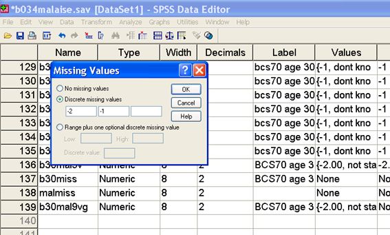

20. Does every little thing get on your nerves
                                                 yes       yes        yes       yes
and wear you out?
21. Does your heart often race like mad?         yes       yes        yes       yes
22. Do you often have bad pain in eyes?          yes       yes        yes       no
23. Are you troubled with rheumatism or
                                                 no        yes        yes       no
fibrosis?
24. Have you ever had a nervous breakdown? no              yes        yes       no

Exercises

Exercise 1. Frequencies

Question 1: How many cohort members were depressed in their thirties? Were more
depressed at age 30 or age 34? (Hint: frequency of b30malg and b34malg variables).

Solution: From the Analyse drop-down menu select Descriptive Statistics and then
Frequencies. Select b30malg b34malg and click on the right arrow button to move the two
variables into the Variable(s) box. Click on OK.

                                                 Teaching resource: 1970 BSC Malaise Inventory | 8 |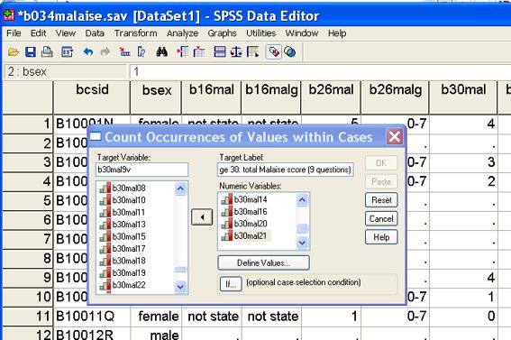

Using syntax: If PASTE is selected instead of OK, a syntax window will open and the
following syntax command will appear in it. Highlight the syntax and then click on the right
arrow button on the toolbar to run the command.

FREQUENCIES
VARIABLES=b30malg b34malg
ORDER= ANALYSIS .

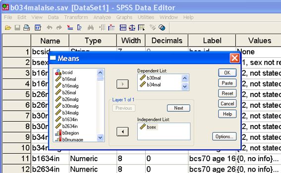
Exercise 2. Means

Question 2: Do men or women have higher mean malaise scores in adulthood? Is the
mean score consistently higher for men or women at age 26, 30 and 34? (Hint: Means of
b26mal b30mal b34mal by bsex)

Solution: From the Analyse drop-down menu select Compare Means and then Means.

Click on b26mal and then b30mal and b34mal and move the variables via the right arrow
button into the Dependent list box. Click on bsex and move into the Independent list box.
Click on OK.

                                                 Teaching resource: 1970 BSC Malaise Inventory | 9 |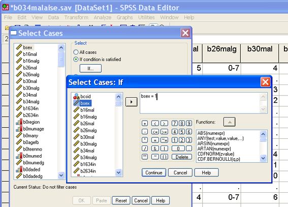

Using syntax: If PASTE is selected instead of OK, a syntax window will open and the
following syntax command will appear in it. Highlight the syntax and then click on the right
arrow button on the toolbar to run the command.

MEANS
TABLES=b26mal b30mal b34mal By bsex
/CELLS MEAN COUNT STDDEV.

Exercise 3. Crosstabs

Question 3: Were cohort members with a low birth weight (

Using syntax: If PASTE is selected instead of OK, a syntax window will open and the
following syntax command will appear in it. Highlight the syntax and then click on the right
arrow button on the toolbar to run the command.

CROSSTABS
/TABLES=b0bwghtg BY b30malg
/FORMAT= AVALUE TABLES
/CELLS= COUNT ROW
/COUNT ROUND CELL.

Question 4: Is there a relationship between family social class and mental well–being? Are
men and women whose father worked in a professional occupation when they were born
more or less likely than those with a father who worked in an unskilled manual job when
they were born to be depressed at age 30? (Hint: the same cross-tab procedure as above
using b0fsoc and b30malg variables).

Question 5: Does academic achievement relate to mental well-being? Are men or women
who have no academic qualifications by age 34 the most likely to be depressed at age 34?
Is the relationship between academic achievement and mental well-being stronger for men
or women? Who is the least likely of all to be depressed at age 34? (Hint: cross-tab of
b34hq5 by b34malg by bsex).

                                               Teaching resource: 1970 BSC Malaise Inventory | 11 |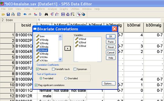

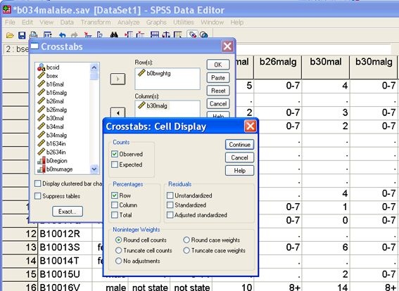
From the Analyse drop-down menu select Descriptive Statistics and then Crosstabs. Select
b34hq5 and click the right arrow button to place the variable into the Row(s) box. Click on
b34malg and click the right arrow button to place into the column(s) box. Click on bsex and
click on the bottom right arrow button and put into the Layer box. Click on the Cells button
and select Row under the percentage heading. Click on the Continue button. Now click on
OK.

Using syntax: If PASTE is selected instead of OK, a syntax window will open and the
following syntax command will appear in it. Highlight the syntax and then click on the right
arrow button on the toolbar to run the command.

CROSSTABS
/TABLES=b34hq5 BY b34malg BY bsex
/FORMAT= AVALUE TABLES
/CELLS= COUNT ROW
/COUNT ROUND CELL.

Exercise 4. Constructing summary scores

Making comparable summary scores at age 30 and age 34

                                               Teaching resource: 1970 BSC Malaise Inventory | 12 |

When all 24 Malaise questions are asked the cut off point to indicate that someone is
experiencing depression is a score of 8+, that is 'yes' was answered to at least 8 questions.
In the survey that took place in 2004 when cohort members were age 34, just 9 of the 24
Malaise questions were asked. A score of 4+ is the cut off point to indicate that someone is
experiencing depression.

In the survey that took place in 2000 when cohort members were age 30 the full 24
questions were asked. A way to test the validity of only using the 9 questions at age 34 is
therefore to see if the same percentage of cohort members are identified as depressed at
age 30 from their responses to the 9 questions as they are from responses to all 24
questions (b30malg).

Question 6: Make an overall score variable from 9 questions at age 30 to match the overall
score variable at age 34. Are the same percentage of men and women identified as
depressed by the reduced number of questions? This can be done through the drop-down
menus or altering some existing syntax. (Hint: in the syntax below replace the variables
starting with b34… with variables starting with b30…. Variable names correspond directly.
For example b34mal02 is the same question as b30mal02).

This is the syntax used to construct the overall malaise score at age 34 (b34mal) and the
grouped variable (b34malg).

count b34mal = b34mal02 b34mal03 b34mal05 b34mal09 b34mal12 b34mal14 b34mal16
b34mal20 b34mal21 (1).

The syntax below maximises the number of cohort members included in the variables by
only excluding those with enough missing values to give them a 'high' (4+) malaise score.

count b34miss = b34mal02 b34mal03 b34mal05 b34mal09 b34mal12 b34mal14 b34mal16
b34mal20 b34mal21 (missing).
compute malmiss =b34mal + b34miss.
if (b34miss > 0 and b34mal = 4) b34mal = -1.
If (b34miss = 9) b34mal = -2.
recode b34mal (0 thru 3=1) (4 thru highest = 2) (-1=-1) (-2=-2) into b34malg.
missing values b34mal b34malg (-1,-2).
variable labels b34mal 'bcs70 age 34: total Malaise score (9 questions)'.
variable labels b34malg 'bcs70 age 34: total Malaise score - grouped'.
value labels b34mal -1'incomplete info' -2'not stated any questions'.
value labels b34malg 1'0-3' 2'4+' -1'incomplete info' -2'not stated any questions'.

freq b34mal b34malg.

Constructing the score from the drop-down menus

STEP 1: Under the Transform drop-down menu, select Count. In the Target Variable box
type in the name of the new summary variable (b30mal9v). In the Target Label box type in
an appropriate label to help identify what the variable is. For example 'BCS70 age 30: total
Malaise score (9 questions)'. Scroll down the list of variables and select the 9 malaise

                                               Teaching resource: 1970 BSC Malaise Inventory | 13 |

variables that are the same as those asked at age 34 (b30mal02, b30mal03, b30mal05,
b30mal09, b30mal12, b30mal14, b30mal16, b30mal20, b30mal21) and click on the right
arrow button to place them in the Variables: box. Once this has been done, click on the
Define Values button.

On the left hand side of the new screen, click on the Value button and enter 1 into the
empty box. Click on the Add button on the right hand side of the screen to move the
information into the Values to Count box. Click on Continue, then OK.

                                               Teaching resource: 1970 BSC Malaise Inventory | 14 |

Using syntax: If PASTE is selected instead of OK, a syntax window will open and the
following syntax command will appear in it. Highlight the syntax and then click on the right
arrow button on the toolbar to run the command.

COUNT
b30mal9v = b30mal02 b30mal03 b30mal05 b30mal09 b30mal12 b30mal14 b30mal16
b30mal20 b30mal21 (1) .
VARIABLE LABELS b30mal9v 'BCS70 age 30: total Malaise score (9 questions)'.
EXECUTE .

STEP 2: Repeat this process to count the number of missing responses for each cohort
member (variable name b30miss). Instead of counting the number of yes (value 1)
responses, select System- or user-missing in the Values to count window.

STEP 3: The next stage is to maximise the number of cohort members we can include in
the new dichotomous variable we will construct (b30mal9vg).

Under the Transform drop-down menu, select Compute. In the Target Variable box type in
the name of the new variable that will add together the number of ‘yes’ responses and the
number of ‘missing’ responses (e.g. malmiss). Scroll down the list of variables to the two
new variables you have just created b30mal9v and b30miss. Select b30mal9v and click on
the right arrow button to move it into the Numeric Expression: box. Click on the + symbol.
Then select b30miss and click on the right arrow button to now move this variable into the
Numeric Expression: box. Once this has been done, click on OK.

                                               Teaching resource: 1970 BSC Malaise Inventory | 15 |

Using syntax: If PASTE is selected instead of OK, a syntax window will open and the
following syntax command will appear in it. Highlight the syntax and then click on the right
arrow button on the toolbar to run the command.

COMPUTE malmiss = b30mal9v + b30miss .
EXECUTE .

STEP 4: Recoding the cohort members who have a valid score in b30mal9v to ‘missing’ if
they did not answer all 9 questions and the number of missing answers could affect
whether they were assigned a depressed label or not in the new dichotomous variable
b30mal9vg.

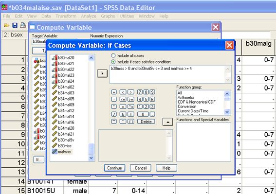
Under the Transform drop-down menu, again select Compute. In the Target Variable box
type in the name of the existing variable b30mal9v. In the Numeric Expression box type in -
1. (We do not want to make a new variable; we are just altering the existing one.) Click on
the If button at the bottom of the screen. A new screen will open. Click on the button Include
if case satisfies condition: Either type in the syntax rules (shown below) or select the
variables from the variable list and click on the right arrow button to move them into the box.
Likewise click on the mathematical symbols and numbers. Click on Continue and then OK.
SPSS will ask if you want to change the existing variable. Click Yes.

                                                Teaching resource: 1970 BSC Malaise Inventory | 16 |

Using syntax: If PASTE is selected instead of OK, a syntax window will open and the
following syntax command will appear in it. Highlight the syntax and then click on the right
arrow button on the toolbar to run the command.

IF (b30miss > 0 and b30mal9v = 4) b30mal9v = -1.
EXECUTE .

Repeat this process to assign a value of -2 to those who did not answer any of the 9
Malaise questions. (HINT: if b30miss = 9, b30mal9v = -2).

Exercise 5. Recoding continuous variables

(continuation of 4.)

STEP 5: Recode the continuous variable into a dichotomous variable.

Under the Transform drop-down menu select Recode and then Into Different Variable.

                                               Teaching resource: 1970 BSC Malaise Inventory | 17 |

Scroll down the list of variables and select b30mal9v, click on the right arrow button to
move the variable into the Numeric variable right arrow Output variable box. Type the name
of the new variable in the Name box, and label in the Label box. Click on the Change button
to move the information into the Numeric variable right arrow Output variable box. Now click
on the Old and New Values button.

                                              Teaching resource: 1970 BSC Malaise Inventory | 18 |

Under Old value select Range and type 0 in the first box and 3 in the second box. Under
New value select Value and type in 1. Click on the Add button to move the information into
the Old right arrow New box. Repeat this for the values in the range 4 – 9 in b30mal9v and
assign 2 as the new value in b30mal9vg. Under Old Value select Value and type in -1.
Under New Value select Copy old value(s), then the Add button. Repeat this to copy the
value -2 to the new variable. Click on Continue, then OK.

Using syntax: If PASTE is selected instead of OK, a syntax window will open and the
following syntax command will appear in it. Highlight the syntax and then click on the right
arrow button on the toolbar to run the command.

RECODE
b30mal9v
(-1=Copy) (-2=Copy) (0 thru 3=1) (4 thru 9=2) INTO b30mal9vg .
VARIABLE LABELS b30mal9vg 'bcs70 age 30: total Malaise score (9 questions - grouped'.
EXECUTE .

STEP 6: Assigning missing values and value labels to b30mal and b34mal9vg. In the
Variable View window, scroll down the variables to b30mal9v and b30mal9vg. Move across
to the Values column and click on the box for b30mal9vg. A new screen will open. Type in 1
in the Value box and 0-3 in the Value Label box. Click on Add. Repeat this for the following
3 values: 2= 4+, -1= incomplete info, -2=not stated any questions. Click on OK.

Assign the same value labels to -1 and -2 in b30mal9v.

                                               Teaching resource: 1970 BSC Malaise Inventory | 19 |

Click on the cell in the Missing column for variable b30mal9vg, and then select Discrete
missing values. Type in -2 and -1 into the separate cells. Repeat this for variables
b30mal9v.

                                               Teaching resource: 1970 BSC Malaise Inventory | 20 |

As you can see, once you know the syntax to write, it is a much faster process than using
the drop-down menus. If you save the syntax file you will also retain a record of how you
made the variables.

Now compare the frequencies of the original Malaise dichotomous variable and the new
dichotomous Malaise variable from the 9 questions. Are the same percentage of cohort
members identified as depressed by the reduced number of questions? (Hint: Frequencies
of b30malg b30mal9vg). Is this the same for men and women? (Hint: run a cross-tab of
b30malg b30mal9vg by bsex).

Exercise 6. Correlations between scores

Question 7: Depression (malaise) is measured at age 16, 26, 30 and 34. At which two time
points, ages, are the scores most strongly associated? Is this the same for men and
women? (Hint: correlate the four continuous variables b16mal b26mal b30mal b34mal).

From the Analyse drop-down menu select Correlate and then Bivariate. Select b16mal and
click the right arrow button to place it into the Variables box. Repeat for variables b26mal,
b30mal, b34mal. Click OK.

Using syntax: If PASTE is selected instead of OK, a syntax window will open and the
following syntax command will appear in it. Highlight the syntax and then click on the right
arrow button on the toolbar to run the command.

                                               Teaching resource: 1970 BSC Malaise Inventory | 21 |

CORRELATIONS
/VARIABLES=b16mal b26mal b30mal b34mal
/PRINT=TWOTAIL NOSIG
/MISSING=PAIRWISE .

Re-run the analyses for men and women separately. (Hint: use Select cases).

From the Data drop-down menu, select Select Cases. Click on If condition is satisfied and
then the If button. Select the bsex variable and click the right arrow button to place it into
the white box. To select men, add = 1 after bsex. Click on Continue and then OK. Now re-
run the Correlate command, first for men then for women. To select women only, add = 2
after bsex.

Using syntax: VALUE LABELS filter_$ 0 'Not Selected' 1 'Selected'.
FORMAT filter_$ (f1.0).
FILTER BY filter_$.
EXECUTE .

                                                Teaching resource: 1970 BSC Malaise Inventory | 22 |

NB: if you are using syntax, a simpler way of selecting men only would be to add the
following instruction before an analysis.

Temporary.
Select if (bsex = 1).
CORRELATIONS
/VARIABLES=b16mal b26mal b30mal b34mal
/PRINT=TWOTAIL NOSIG
/MISSING=PAIRWISE .

Exercise 7. Linear regression

Linear regression estimates the coefficients by a linear equation, involving one or more
independent variables, which best predict the value of the dependent variable, in this
example malaise score at age 34.

Question 8: Although the correlation between malaise scores at age 16 and 34 was the
weakest among the four scores, the positive correlation was highly significant. Using simple
linear and then multiple regression we first predict a high malaise score at age 34 from
malaise score at age 16, and then control for birthweight, gender, mother’s age of leaving
full-time education and age left full-time education.

From the Analyse drop-down menu select Regression and then Linear. Select b34mal and
click the right arrow button to place it into the Dependent box. In the same way, add b16mal
bsex b0bwght b0mumed and b34lefted to the Independent(s) box.

Click on Statistics and select Descriptive Statistics and Casewise Diagnostics – this will
identify any outliers in the data.

Click on Plots to request a plot of Standardised Predicted Residuals (Y) against
Standardised Predicted Values (X).

The following syntax is produced when the paste command is selected.

Using syntax: If PASTE is selected instead of OK, a syntax window will open and the
following syntax command will appear in it. Highlight the syntax and then click on the right
arrow button on the toolbar to run the command.

REGRESSION
/DESCRIPTIVES MEAN STDDEV CORR SIG N
/MISSING LISTWISE
/STATISTICS COEFF OUTS R ANOVA
/CRITERIA=PIN(.05) POUT(.10)
/NOORIGIN
/DEPENDENT b34mal
/METHOD=ENTER b16mal /METHOD=ENTER b16mal bsex b0bwght b0mumed b34lefted
/SCATTERPLOT=(*ZPRED ,*ZRESID )

                                                Teaching resource: 1970 BSC Malaise Inventory | 23 |

/CASEWISE PLOT(ZRESID) OUTLIERS(3).

Fitting real data into the Linear regression equation

The Linear Regression equation is:

(Predicted) Ȳ = b0 = b1(x1) + b2(x2) +……..bp(xp)

Using the regression equation (above), use the statistics produced in the B column in the
Coefficients table in the SPSS output file and the information below to calculate the
estimated Malaise score for a cohort member at age 34.

This particular cohort member

   •   is female
   •   had a low birth weight of 2410 grams
   •   had a very high malaise score at age 16 of 44
   •   had a mother who left education at age 15
   •   had an A/S level qualification (highest academic qualification achieved)

Using syntax: SPSS syntax to identify this cohort member is temporary.

select if (bsex = 2 and b16mal = 44 and b0mumed = 15 and b0bwght = 2410 and b34hq13
= 4).
SUMMARIZE
/TABLES=bcsid bsex b16mal b0mumed b0bwght b34hq13. /FORMAT=VALIDLIST
NOCASENUM TOTAL LIMIT=100
/TITLE='Case Summaries'
/MISSING=VARIABLE
/CELLS=COUNT .

Compare this with their actual Malaise score at age 34 (Y). How accurate was the predicted
Y? (Hint: to find the individual cohort member in the data file, go to the Data View window
and place the cursor on the bcsid column, select Find from the Edit drop-down menu. The
bcsid number to find is B24447M. Look under b34mal to see the actual score obtained at
age 34).

                                                Teaching resource: 1970 BSC Malaise Inventory | 24 |

You could repeat the above analysis using different but similar variables in the data file. For
example, replace highest qualification at age 34 with the age the cohort member left full-
time education (b34lefted), mother's age of leaving full-time education with father's age of
leaving full-time education (b0daded) or family social class at some point in childhood
(b0psoc, b5psoc, etc).

Exercise 8. Logistic regression

A similar analysis can be run using logistic regression to predict depression at age 34 from
signs of depression at age 16, birth weight, gender, mother’s age of leaving full-time
education and own highest qualification by age 34.

From the Analyse drop-down menu select Regression and then Binary Logistic to open the
Logistic Regression dialog box. Transfer the categorical Malaise score variable b34malg
into the Dependent box, and the (predictor) variables into the Covariates box. In the first
analysis just move the grouped malaise score at age 16 (b16malg). In the second stage of
the analysis include the other measures from birth using the categorical (that is, not
continuous) measures for mother in education post-15 (b0mumedg), birth weight
(b0bwghtg), gender (bsex) and highest qualification at age 34 (b34hq5).

Reference Category
Categorical variables require a reference category to be set. There are different methods of
contrasting category membership in a variable. The default method in SPSS is Indicator,
with the last (highest value) category being set as the reference category. (In the SPSS
output, the reference category is represented in the contrast matrix as a row of zeros.)

                                                Teaching resource: 1970 BSC Malaise Inventory | 25 |

In our model, this would mean that the reference category in the variable b34hq5 would be
set as category 5'higher degree / PGCE'. The relative importance of membership to each of
the other qualification groups (values 0'none' up to 4'degree….nursing qual') will be
compared against membership to category 5'higher degree / PGCE'.

Click on the Categorical button to open the Define Categorical Variables box. Move the
covariates into the Categorical Covariates box. The default makes the last (highest value)
category of a variable the reference category. To change the reference category to the first
(lowest value) category, click on First and then Change. Do this for the each of the following
variables b16malg, bsex, b0bwghtg, b0meumedg. Click on Continue and then OK.

Using syntax: If PASTE is selected instead of OK, a syntax window will open and the
following syntax command will appear in it. Highlight the syntax and then click on the right
arrow button on the toolbar to run the command.

Initial analyses
LOGISTIC REGRESSION b34malg
/METHOD = ENTER b16malg
/CONTRAST (b16malg)=Indicator(1)
/CRITERIA = PIN(.05) POUT(.10) ITERATE(20) CUT(.5) .

                                               Teaching resource: 1970 BSC Malaise Inventory | 26 |

Second analyses
LOGISTIC REGRESSION b34malg
/METHOD = ENTER b16malg bsex b0mumedg b0bwghtg b34hq5
/CONTRAST (b16malg)=Indicator(1) /CONTRAST (bsex)=Indicator(1) /CONTRAST
(b0mumedg)=Indicator(1) /CONTRAST
(b0bwghtg)=Indicator(1) /CONTRAST (b34hq5)=Indicator
/CRITERIA = PIN(.05) POUT(.10) ITERATE(20) CUT(.5) .

Looking at the Variables in the Equation table:

   •       How much more likely were depressed teenagers to grow up to be a depressed 34
           year old?
   •       After taking into account gender, birth weight, whether mother remained in
           education after 15 and own highest qualification, how much more likely were
           depressed teenagers to grow up to be depressed at age 34?
   •       After malaise score at age 16, which variable makes the biggest contribution to the
           model?

Further stages of analysis

Repeat the above analysis adding in new variables or replacing variables with similar
measures. For example, whether father remained in education post-15 (b0dadedg).
Remember to think about whether it makes more sense to set the first or last category as
the reference category. If a variable has many categories (e.g. family social class), recode
to have fewer categories.

   •       Is mother's or father's age of leaving full-time education the stronger measure
           (bigger coefficient) for predicting depression at age 34?
   •       Which variable makes a significant contribution to the model when mother's age of
           leaving full-time education is included, but not when father's age of leaving full-time
           education is included?

You could also try repeating the above analyses for men and women separately.

       •     Are the results the same for men and women separately?

Interaction Terms

For each variable in the logistic model, it is assumed that the effect is the same for all
values of other variables in the model. For example, the effect of level of a mother’s
education is the same for men as it is for women. If this is not the case, there is an
interaction. You can include a term for the level of mother’s education (b0mumedg) by
gender (bsex) interaction in your model.

To include an interaction term between depression at age 16 and gender in your model
click on bsex and then b16malg whilst simultaneously pressing the Ctrl key on your PC
keyboard. This will mean both variables are highlighted. Click on the >a*b> button to place
an interaction term in the Covariates dialog box. Continue as before.

                                                    Teaching resource: 1970 BSC Malaise Inventory | 27 |

Using syntax: If PASTE is selected instead of OK, a syntax window will open and the
following syntax command will appear in it. Highlight the syntax and then click on the right
arrow button on the toolbar to run the command.

LOGISTIC REGRESSION b34malg
/METHOD = ENTER b16malg bsex b0mumedg b0bwghtg b34hq5 b16malg*bsex
/CONTRAST (b16malg)=Indicator(1) /CONTRAST (bsex)=Indicator(1) /CONTRAST
(b0mumedg)=Indicator(1) /CONTRAST
(b0bwghtg)=Indicator(1) /CONTRAST (b34hq5)=Indicator
/CRITERIA = PIN(.05) POUT(.10) ITERATE(20) CUT(.5) .

      •   Is the interaction significant? Try repeating this using the continuous malaise
          score at age 16 variables (b16mal). Are the same results obtained?

Remember all of these exercises can be repeated for cross-cohort comparisons using
similar variables in the NCDS data file n042malaise.sav.

References
Bennett, K.E. and Haggard, M.P. (1999) ‘Behaviour and cognitive outcomes from middle
ear disease’. Archives of Disease in Childhood, 80(1), pp.28-35.

                                                Teaching resource: 1970 BSC Malaise Inventory | 28 |

Bowling, A. (1983) Initial analyses with the malaise inventory, NCDS4 Working Paper 2,
London: SSRU, City University.

Buchanan, A., Flouri, E. and Ten Brinke, J. (2002) ‘Emotional and behavioral problems in
childhood and distress in adult life: risk and protective factors’, Australian and New Zealand
Journal of Psychiatry, 36(4), pp.521-527.

Buchanan, A., Ten Brinke, J. and Flouri, E. (2000) ‘Parental background, social
disadvantage, public care and psychological problems in adolescence and adulthood’,
Journal of the American Academy of Child and Adolescent Psychiatry, 39(11), pp.1415-
1423.

Bynner, J., Woods, L. and Butler, N.R. (2002) Youth factors and labour market experience
in job satisfaction, CLS Cohort Studies Working Paper No 3. London: SSRU, City
University.

Chase-Lansdale, P.L., Cherlin, A. and Kiernan, K.E. (1995) ‘The long-term effects of
parental divorce on the mental health of young adults: a developmental perspective’,
Journal of Child Development, 66(6), pp.1614-1634.

Cheung, S.Y. and Buchanan, A. (1997) ‘Malaise scores in adulthood of children and young
people who have been in care’, Journal of Child Psychology and Psychiatry and Allied
Disciplines, 38(5), pp.575-580.

Cheung, Y.B. (2002) ‘Early origins and adult correlates of psychosomatic distress’, Social
Science and Medicine, 55(6), pp.937-948.

Collishaw, S., Maughan, B. and Pickles, A. (1998) ‘Infant adoption: psychosocial outcomes
in adulthood’, Social Psychiatry and Psychiatric Epidemiology, 33(2), pp.57-65.

Flouri, E., Buchanan, A. and Brem, V. (2000) ‘In and out of emotional and behavioural
problems’ in Buchanan, A. and Hudson, B.L (eds.), Promoting children's emotional well-
being, Oxford: Oxford University Press.

Flouri, E. and Buchanan, A. (2003) ‘The role of father involvement in children's later mental
health’, Journal of Adolescence, 26(1), pp.63-78.

Flouri, E. (2004) ‘Subjective well-being in midlife: the role of involvement of and closeness
to parents in childhood’, Journal of Happiness Studies, 5(4), pp.335-358.

Grant, G., Nolan, M., and Ellis, N. (1990) ‘A Reappraisal of the Malaise Inventory’, Social
Psychiatry and Psychiatric Epidemiology, 25(4), pp.170-178.

Hirst, M.A. (1983) ‘Evaluating the Malaise Inventory: an item analysis’, Social Psychiatry,
18, pp.181-184.

Hobcraft, J. and Kiernan, K.E. (1999) Childhood poverty, early motherhood and adult social
exclusion, CASE Paper No 28. London: STICERD-LSE-ESRC Centre for the Analysis of

                                                Teaching resource: 1970 BSC Malaise Inventory | 29 |

Social Exclusion, LSE.

Hobcraft, J. (2000) The roles of schooling and educational qualifications in the emergence
of adult social exclusion, CASE Paper No 43. London: STICERD-LSE-ESRC Centre for the
Analysis of Social Exclusion, LSE.

Clegg, J. et al. (2005) ‘Developmental language disorders - a follow-up in later adult life.
Cognitive, language and psychosocial outcomes’, Journal of Child Psychology and
Psychiatry and Allied Disciplines, 46(2), pp.128-149.

Hope, S., Rodgers, B. and Power, C. (1999) ‘Marital status transitions and psychological
distress: longitudinal evidence from a national population sample’, Psychological Medicine,
29, pp.381-389.

McGee, R., Williams, S., and Silva, P. A. (1986) ‘An evaluation of the Malaise Inventory’,
Journal of Psychosomatic Research, 30(2), pp.147-152.

Power, C., Hertzman, C., Matthews, S. and Manor, O. (1997) ‘Social differences in health:
life-cycle effects between ages 23 and 33 in the 1958 British birth cohort’, American Journal
of Public Health, 87(9), pp.1499-1503.

Power, C. and Manor, O. (1992) ‘Explaining social class differences in psychological health
among young adults: a longitudinal perspective’, Social Psychiatry and Psychiatric
Epidemiology, 27(6), pp.284-291.

Rodgers, B. et al. (1999) ‘Validity of the Malaise Inventory in general population samples’,
Social Psychiatry and Psychiatric Epidemiology, 34(6), pp.333-341.

Rutter, M., Tizard, J., and Whitmore, K. (1970) Education, health and behaviour, London:
Longmans.

Sacker, A. and Cable, N. (2006) ‘Do adolescent leisure-time physical activities foster health
and well-being in adulthood? Evidence from two British birth cohorts’, European Journal of
Public Health, 16(3), pp.331-335.

Steptoe, A. and Butler, N.R. (1996) ‘Sports participation and emotional well-being in
adolescents’, Lancet, 347(9018), pp.1789-1792.

Acknowledgements
UK Data Service would like to thank the Centre for Longitudinal Studies, Institute of
Education, University of London for their permission to reproduce this resource online.
.

                                                Teaching resource: 1970 BSC Malaise Inventory | 30 |

Teaching resource: 1970 BSC Malaise Inventory | 31 |