Text-Based Insights into Stock Market Behavior - Professor Steven J. Davis ABFER Industry Outreach Dialogue
←
→
Page content transcription
If your browser does not render page correctly, please read the page content below
Text-Based Insights into
  Stock Market Behavior

    Professor Steven J. Davis

ABFER Industry Outreach Dialogue
    Singapore, 2 August 2018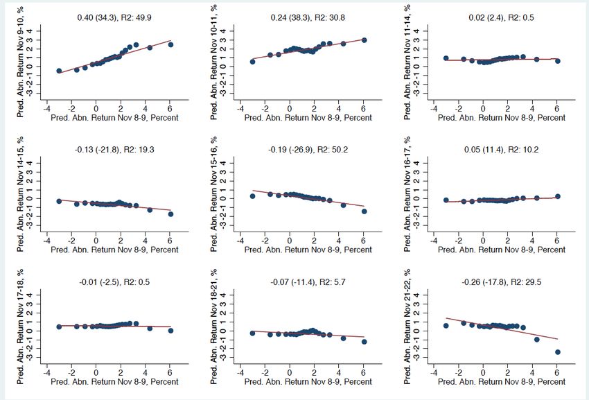
Abstract
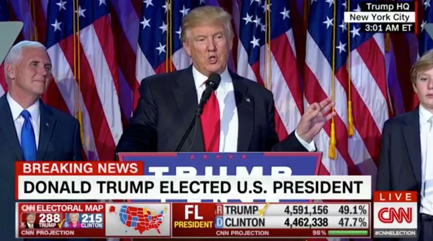
U.S. stocks rose sharply in reaction to Donald Trump’s
surprise victory in the November 2016 presidential election. The
boom perplexed many analysts, including prominent economists
who had predicted a market crash if Trump won.
To throw light on the market reaction, I look to firm-level
equity returns in the wake of the election. In particular, I relate
firm-level returns to text-based measures of their exposures to
government policy and regulatory risks. I construct these
measures using text in their mandatory 10-K filings.
While average returns responded positively to Trump’s win
(and Clinton’s loss), firm-level reactions vary enormously. For
example, firms with high exposure to regulatory risks enjoyed
especially high returns on 9 November and the next 2 days,
while firms with high exposure to healthcare policy risks saw
large relative and, in some cases, absolute equity price drops.
The results suggest that equity prices do not immediately
and fully adjust to surprise events that (a) involve unusual shifts
in the structure of price-relevant risks and (b) require large
information processing resources to fully assess.
2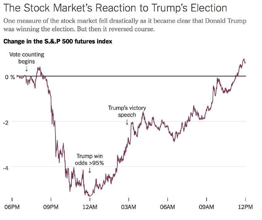
Text as Data
My remarks today draw on two projects that use
text as data to develop new insights into stock
market behavior and economic performance.
• “What Triggers Stock Market Jumps?” with Scott
  Baker, Nick Bloom and Marco Sammon.
   – Human readings of newspaper articles about
     thousands of large daily jumps in national equity
     markets for 14 countries.
   – Key result for today’s talk: News from and about
     the United States triggers national stock market
     jumps around the globe.
• “Diagnosing the Stock Market Reaction to Trump’s
  Surprise Election Victory,” with Cristhian Seminario
   – Automated readings of about 61,000 regulatory
     filings with the U.S. Securities and Exchange
     Commission.
                                                         3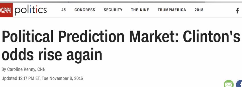
Coding National Equity Market Jumps
1. Set daily jump threshold: Aim for about 1% of daily moves
    à a threshold of |2.5%| for most countries.
2. Pull dates with market moves > threshold
3. Use own-country newspaper articles to code jumps
   A. Go to online newspaper archive
   B. Enter newspaper, date range (next day) and search
       criteria (e.g., “stock market”)
   C. Select article
4. One or more humans read and code the article(s),
    according to our coding guide.
   – Rely on native-language speakers to code articles.
5. Record the jump reason per the journalist, the geographic
    source of the news that triggered the jump, journalist
    confidence in the jump explanation, and more.
                                                          4
Key Result for Today’s Talk U.S. developments trigger a huge share of equity market jumps across the globe. – Excluding data for the United States, leading local newspapers attribute 34% of jumps in their national stock markets to news from or about the U.S. – The U.S. role in this regard dwarfs the role of Europe, China and other large regions and countries. – The U.S. role is especially pronounced during the Global Financial Crisis.
Share of Jumps Attributed to U.S. Developments
   .8

         Excluding jumps in U.S. stock market

                                            .8
                                                                               Global
                                                                Tech Boom/     Financial
           Early 1980’s                                         Bust           Crisis
   .6

                                            .6

                                                                                                  US Share of Global GDP
           recession
                        US Share of Jumps
                      1987 Crash

                                            .4
                                                        Asian/LTCM
   .4

                                                        crises

                                                                             Eurozone
                                            .2

                                                                             Crisis
   .2

                          Gulf War I
                                            0

                                                 1980           1990           2000              2010

                                                          U.S. Jump Share       U.S. GDP Share
    0

        1980                                1990                   2000                 2010

Notes: Average share of jumps attributed to U.S. developments by year in Australia, Canada,
China (HK), China (Shanghai), Germany, Greece, Ireland, Japan, New Zealand, Saudi Arabia,
Singapore, South Africa, South Korea and UK. Dot size is proportional to the average number of
jumps by country/year. U.S. Share of PPP-adjusted global GDP using IMF data.
News about the U.S. Moves Equity Markets
Much More than News about Europe
The sample for “US Jump Share” excludes the United States.
.8
The sample for “Europe Jump Share” excludes European countries
.6
.4
.2
0
1980 1990 2000 2010
Europe Jump Share US Jump Share
Europe GDP Share US GDP Share
GDP shares computed using contemporaneous exchange rates.Why the Outsized Role for the U.S.?
1. The U.S. has been the chief architect and guarantor of the
global economic and security order since WW II.
2. It remains the world’s foremost military power.
3. Most international trade is invoiced in a few currencies,
mainly the Dollar.
4. Many countries tie their currency values to the Dollar.
5. The Dollar is the world’s dominant reserve currency.
6. The U.S. is the world’s major supplier of safe, liquid debt.
7. Much of the world’s offshore bank lending is in Dollars.
8. Portfolio investors around the world exhibit a strong
preference for dollar-denominated securities.
9. The Fed is the world’s leading monetary policymaker.
10. It’s also the world’s chief central bank, as illustrated by Fed
swap lines with other central banks during and after the GFC.
8Turning to the U.S.
stock market …
… and its reaction
to Donald Trump’s
surprise election
as U.S. President
9Noon on Election Day! Washington (CNN) Hillary Clinton's odds of winning the presidency rose from 78% last week to 91% Monday before Election Day, according to CNN's Political Prediction Market.
A big surprise!
Initially, stocks fell sharply in after-hours trading

From “Markets Sent a Strong Signal on Trump … Then Changed Their Minds,” Justin
Wolfers, New York Times, 18 November 2016
But Stocks Boomed on 9 November
Histogram of Daily Market Returns, U.S. Stocks
    Sample Period: 8 November 2016 +/- 360 Days

                                               Trump Election
                              Trump Election
  Using
  Closing
  Prices
… Confounding Prominent Economists Justin Wolfers, New York Times, 18 November 2016: “Throughout the campaign, stocks rose whenever campaign developments made it less likely that Mr. Trump would be elected.” This assessment rests on Wolfers’ pre-election empirical study with Erik Zitzewitz. Their bottom line: “[W]e estimate that market participants believe that a Trump victory would reduce the value of the S&P 500, the UK, and Asian stock markets by 10-15%.”
Our Approach: Examine the Cross-
Section of Abnormal Equity Returns
in Reaction to Trump’s Victory
1. Trump and Clinton were far apart on many policy
   issues: regulation, healthcare, trade, etc. Not a
   Tweedledee vs. Tweedledum election!!
2. Firms differ in their exposures to policy risks.
3. Quantify these risks using Part 1a (“Risk
   Factors”) of listed firms’ annual 10-K filings.
4. Trump’s surprise victory abruptly shifted the level
   and structure of important policy risks.
5. We look to the cross-section of firm-level returns
   to assess the effects of that shift and gain insight
   into the market’s reaction to Trump’s win.
The Cross-Firm Dispersion of Abnormal Returns
 Was Very High in the Wake of Trump’s Victory
Histogram of Cross-Firm St. Dev. of Daily Abnormal Returns
      Sample Period: 8 November 2016 +/- 360 Days
                Abnormal (CAPM)

                                       Trump Election

                                                        Trump Election
                returns based on
                data for 360 days
                before the election.
Analysis Sample • Common equity securities (primary issue) traded on AMEX, NYSE and NASDAQ of firms incorporated in the United States, with prices quoted in U.S. Dollars. • Daily closing prices, shares outstanding and shares traded from Compustat North America, with adjustments for stock splits, reverse splits, dividends, etc. Market return data from Ken French’s website. • Sample period: ±360 calendar days from Nov 8, 2016 • 3,606 firms with closing prices on 8 and 9 November. • Matched to 3,383 firms with at least one 10-K filing (with non-empty Part 1a) from January 2006 to July 2016. – Part 1a is not obligatory for all listed firms. • Drop 102 firms with no NAICS code. Drop 20 with fewer than 126 daily return observations in pre-election window. • 3,261 firms in the final sample. – About 1.5 million daily return observations 17
Part 1A of the 10-Ks
• Since 2006 (for FY 2005) the SEC requires most publicly
  held firms to include a separate discussion of “Risk Factors”
  in Part 1a of their annual 10-K filings.
• In explaining “How to Read a 10-K” at
  www.sec.gov/answers/reada10k.htm, the SEC describes
  Part 1a as follows:
   – Item 1A - “Risk Factors” includes information about the
     most significant risks that apply to the company or to its
     securities. Companies generally list the risk factors in
     order of their importance. In practice, this section focuses
     on the risks themselves, not how the company addresses
     those risks. Some risks may be true for the entire
     economy, some may apply only to the company’s industry
     sector or geographic region, and some may be unique to
     the company.                                              18
How We Use the 10-Ks 1. Develop term sets that correspond to various policy risk categories. Examples: Tax policy, trade policy, government spending, healthcare policy, financial regulation, etc. 2. For each 10-K filing – and each term set – calculate the percentage of sentences in Part 1a with one or more terms in the set. 3. Average the percentage over available years for each firm and term set to get our risk exposure measures. 19
A Warm-Up Investigation
1. For each 10-K filing with a non-empty Part 1a:
   – Calculate the percentage of sentences in Part 1a
      that contains “regulation,” “regulate” or “regulatory.”
   – Average this percentage over years for each firm.
2. This average value is our measure of Raw Regulation
   (Risk) Exposure for the firm.
3. Compute the firm’s daily return as 100 X log change in
   the closing price from November 8 to November 9.
4. Obtain the CAPM abnormal return for each firm from
   November 8 to 9.
5. Relate Raw Regulation Exposure to abnormal equity
   returns in reaction to Trump’s surprise election victory.
6. Plot the firm’s daily return against its Raw Regulation
   Exposure.
                                                                20
Firms with greater exposure to regulatory risks
had higher abnormal returns on 9 November
The estimated cross-sectional effect is large:
Multiplying the slope coefficient by the IQR of
the Raw Regulation Exposure measure (7.6
percentage points) implies a daily return
differential of 1.2 percentage points.
(Abnormal) Returns on 9 November:
Mean Firm-Level Daily Return: 1.1%
IQR of Daily Returns: 4.4%Extending Our Approach
1. Relate firm-level (abnormal) equity returns on
9 November 2016 to a range of policy risks.
2. Consider 20+ distinct policy risk categories.
3. Measure each firm’s policy risk exposures
using text from 10-K filings in the years before
the election.
4. Use multiple regression models to estimate
firm-level stock returns on November 9 as a
function of their policy risk exposures.
22Full Set of Policy Risk Categories
• Regulation (6 categories): Labor, financial, intellectual
property, environmental and energy, food and drug,
generic and other regulation
• Taxes (8 categories): Individual income taxes, business
profit taxes, business tax credits, tax treatment of
foreign earnings, tax-filing services, property taxes,
sales and excise taxes, generic and other taxes.
– A strikethrough denotes a category we consider but
do not use in our preferred statistical model.
• Entitlement and welfare programs
• Government purchases and fiscal policy
• Government-sponsored enterprises
• Monetary policy
• Healthcare policy
• Trade and exchange rate policy 23Example: The Term Set for
Financial Regulation
Financial Regulation: {bank supervision}, {thrift
supervision}, {financial reform}, {truth in lending},
{firrea}, {Glass-Steagall}, {Dodd-frank}, {tarp, Troubled
Asset Relief Program}, {Volcker rule}, {Basel}, {stress
test}, {deposit insurance, fdic}, {federal savings and
loan insurance corporation, fslic}, {office of thrift
supervision, ots}, {comptroller of the currency, occ},
{commodity futures trading commission, cftc},
{Financial Stability Oversight Council}, {house financial
services committee}, {Bureau of Consumer Financial
Protection, Consumer Financial Protection Bureau,
CFPB}, {SBA loan program}What Do We Find?
• Our policy risk exposure measures account for more than
20% of firm-level return differences on 9 November 2016.
• Firms with greater exposure to regulatory risks had higher
(abnormal) equity returns on 9 November.
– An exception: Greater exposure to regulations that
favor “green” jobs and energy sources.
• Firms with greater exposure to risks associated with
Labor Regulation, Food and Drug Policy, and IP Policy
had especially high returns on 9 November.
• Healthcare delivery firms and those with high exposures
to healthcare policy risks had poor returns on November
9 in relative terms and, in some case, absolute terms.
• Firms with greater exposure to risks associated with
Trade Policy, Entitlement and Welfare Programs, and
Government-Sponsored Enterprises had lower returns.
The next few slides illustrate some of these resultsPartial Regression Scatter Plots for Firm-Level
Stock Returns on 9 November 2016
Observations binned on variable
on horizontal axis, controlling for
other regressors.Coefficient (t-stat) on Healthcare Industry Dummy: -1.6 (-5.5)
Coefficient (t-stat) on Green
Industry Dummy: -0.8 (-4.0).
BLS Green designations.
A Slow Market Reaction
The stock market did not fully digest the implications of the
election outcome by market close on 9 November.
• Instead, (conditional) firm-level abnormal returns over
   the next 2 trading days strongly reinforced the initial
   market response to the election surprise.
• The shift in (conditional) firm-level abnormal returns
   over the next 2 trading days was 65% as large as the
   initial reaction on 9 November.
   – See charts on the next slide.
   – We exclude firms with very small market caps for this
       analysis. Including them yields very similar results,
       except it takes 3 trading days after 9 November for
       the market to fully price the election outcome.
Stock Prices Continued Moving in the Same Direction over the Next 2 Trading Days How we construct these two charts: 1. Fit our regression model separately to firm-level returns on November 9, 10 and 11, letting the coefficients vary freely across days. 2. For each trading day, recover the model’s predicted values for each firm. 3. Plot the predicted values for November 10 (left chart) or November 11 (right) on the predicted values for November 9. 4. To improve visual clarity, group the firm-level data into 20 bins defined on predicted returns for 9 November. The reported coefficient (t-statistic) and R-squared values are for the underlying firm-level regression.
Similar Market Behavior on Other Days?
  No!
 1. We reran our regression model on each day in a one-year
    window before 8 November 2016 (election day).
 2. We find no evidence that daily firm-level equity returns
    respond systematically to policy risk exposures before the
    election.
 3. The same conclusion holds for the 3 best and the 3 worst
    market days in the one-year pre-election window.

 What does this mean?
 • Our results for 9 November 2016 do not reflect some
   omitted factor that is systematically related to daily firm-
   level equity returns.
 • Trump’s surprise election victory shifted firm-level equity
   prices in an unusual manner.
Summing Up & Taking Stock
1. The election surprise triggered a large, positive stock
market response on 9 November, strongly contradicting
pre-election assessments of how market would react.
2. The structure of firm-level equity returns on 9 November
was highly dispersed, highly unusual, and clearly tied to
firm-level policy risk exposures, as derived from 10-Ks.
– Firms with high exposures to regulatory risks saw
especially high equity returns on 9 November
– Healthcare delivery firms and those with high
exposures to healthcare policy risks fared poorly in
relative terms and, in some case, in absolute terms.
3. The stock market did not fully digest the implications of
the election outcome by market close on 9 November. It
took 2 more trading days to fully price the election.4. These results suggest that equity prices do not immediately
and fully adjust to surprise events that (a) involve unusual
shifts in the structure of price-relevant risks and (b) require
large information processing resources to fully assess.
– Human collection and processing of available
information is costly, and it takes time. Thus, the surprise
realization of events that satisfy (a) and (b) need not be
fully and immediately incorporated into equity prices.
– This explanation might sound like common sense. But
it’s at odds with the Efficient Markets Hypothesis, which
says that stock prices quickly adjust to publicly available
information. A pricing response that settles in over 3
trading days is not quick.
5. Asset price responses to prediction-market probability
changes are unreliable guides to the actual price effects of
major surprise outcomes when (a) and (b) hold.You can also read