The Astronomer's Theory of Everything
←
→
Page content transcription
If your browser does not render page correctly, please read the page content below
The Astronomer’s Theory of Everything

                      David W. Hogg
Center for Cosmology and Particle Physics, New York University

                    2013 September 19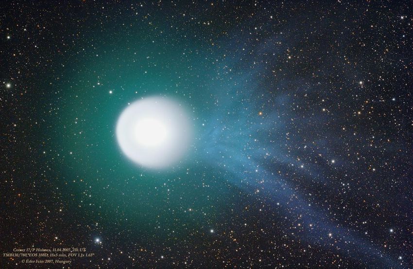
Data-Science and Engineering for Huge
            Astrophysics Projects

                      David W. Hogg
Center for Cosmology and Particle Physics, New York University

                    2013 September 19
Nuisance parameters

                      David W. Hogg
Center for Cosmology and Particle Physics, New York University

                    2013 September 19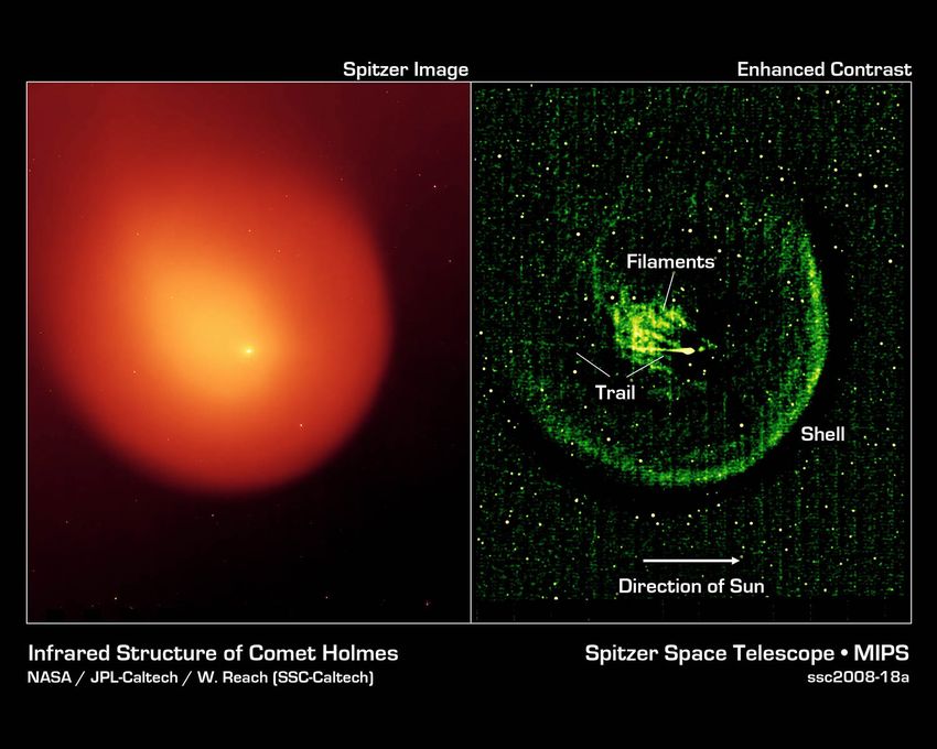
Principal collaborators

     I   Jo Bovy (IAS)
     I   Rob Fergus (NYU CS)
     I   Dan Foreman-Mackey (NYU)
     I   Dustin Lang (CMU)
     I   Sam Roweis (deceased)
Comprehensive astrophysics

    I   Position of “every” galaxy and quasar out to some high
        redshift.
    I   Amplitude of “every” large-scale structure mode inside the
        Hubble volume.
    I   Position, velocity, and chemistry of “every” star in the Milky
        Way Galaxy.
    I   Composition and semimajor axis of “every” planet in the Solar
        Neighborhood.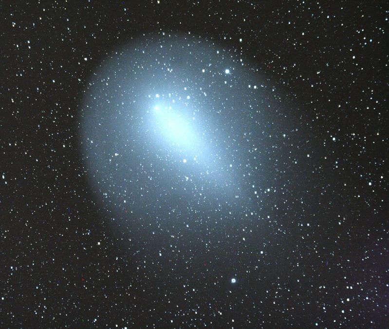
take-home message

    I   You have to build a probabilistic model of the data, and that
        model has to explain and include many parts of the problem
        you don’t care about.
example 1: quasar target selection

     I   SDSS-III BOSS and SDSS-IV eBOSS aim to take spectra of a
         significant fraction of all the quasars in the Universe.
     I   Quasars are hard to tell apart from stars.
     I   XDQSO is the best current method.
           I   build a data-driven model of the stars and the quasars
           I   build a causal, physical model of the photometric noise
                 I   Bovy, J., et al., 2011, Think outside the color-box:
                     Probabilistic target selection and the SDSS-XDQSO quasar
                     targeting catalog, Astrophys. J. 729 141.
                 I   Bovy, J. et al., 2012, Photometric redshifts and quasar
                     probabilities from a single, data-driven generative model,
                     Astrophys. J. 749 41.
What’s a data-driven model?

    I   “The data are the model.”
    I   very flexible forms
          I   histograms—one parameter per bin
          I   images—one parameter per pixel (or more)
          I   mixtures of Gaussians
    I   non-parametrics
          I   model size grows with the data
          I   infinite dimensional in some sense
          I   heavily regularized
XDQSO target selection (Bovy et al., 1011.6392)
example 2: exoplanets with Kepler

    I   (The Kepler Satellite broke last May; our best people are on
        it!)
    I   Kepler has found thousands of exoplanets, and future
        Kepler -like missions will find many thousands more.
    I   Planet transits (of greatest interest) require sensitivity to brief
        events at the 10−5 level.
    I   Typical stars and telescopes vary by much more than this.
          I   build a data-driven model of the stellar variability
          I   build a causal, physical model of the Spacecraft
                I   Hogg, D. W. et al., 2013, Maximizing Kepler science return
                    per telemetered pixel: Detailed models of the focal plane in
                    the two-wheel era, arXiv:1309.0653
                I   Montet, B. T. et al., 2013, Maximizing Kepler science return
                    per telemetered pixel: Searching the habitable zones of the
                    brightest stars, arXiv:1309.0654
modeling Kepler lightcurves
modeling the Kepler focal plane

                                                       1.05
                  True Subpixel Flat-field
    20
    15
    10                                                 1.00
     5
    0
         0   10   20     30       40         50   60
                                                       0.95
modeling the Kepler focal plane
1.05
Learned Subpixel Flat-field
20
15
10 1.00
5
0
0 10 20 30 40 50 60
0.95modeling the Kepler focal plane
0.05
(True - Learned) Subpixel Flat-field
20
15
10 0.00
5
0
0 10 20 30 40 50 60
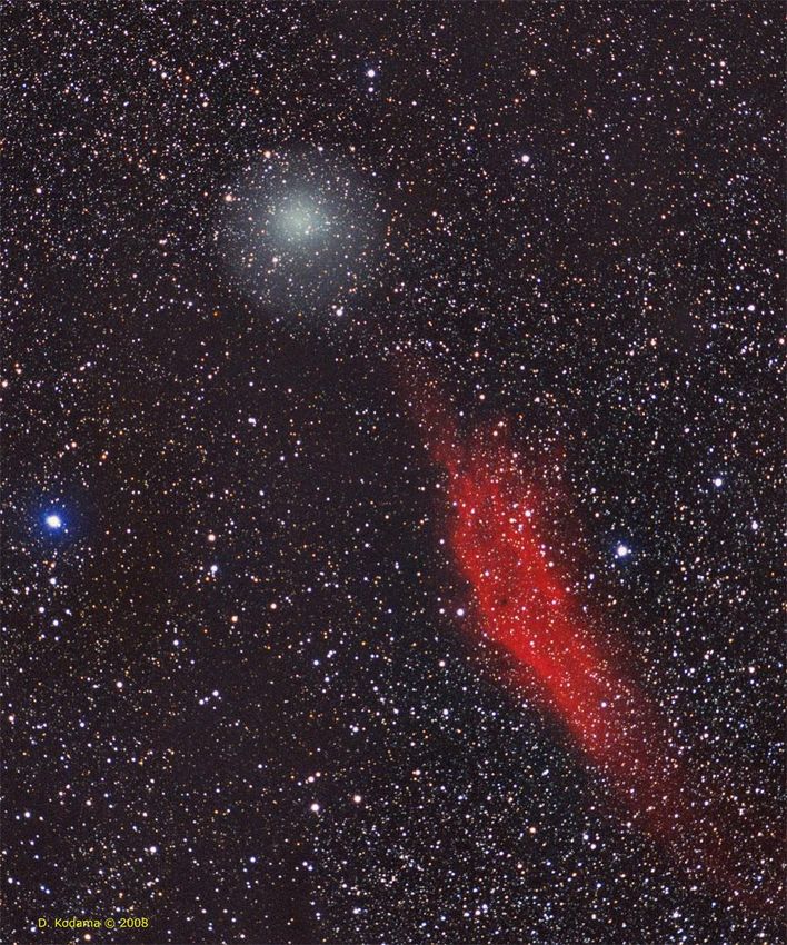
0.05example 3: the Web as a sky survey
I There are hundreds of thousands (at least) of astronomically
relevant images on the Web.
I Most of it is in archival disarray.
I To use it, we have to understand how and why it was taken.
I build a data-driven model of the motivations of the
photographers
I build a causal, physical model each individual image
I Lang, D. et al., 2010, Astrometry.net: Blind astrometric
calibration of arbitrary astronomical images, Astron. J. 139
1782–1800.
I Barron, J. T. et al., 2008, Cleaning the USNO-B Catalog
through automatic detection of optical artifacts, Astron. J.
135 414–422.
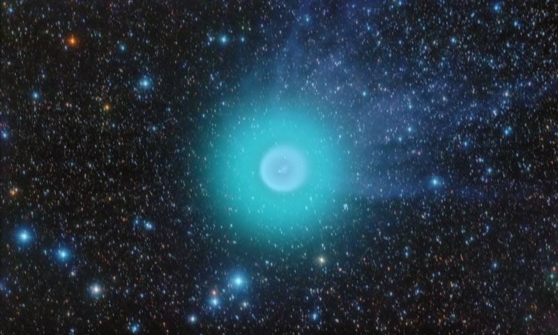
I Lang, D. & Hogg, D. W., 2012, Searching for comets on the
World Wide Web: The orbit of 17P/Holmes from the behavior
of photographers, Astron. J. 144 46.search “Comet Holmes” on Yahoo!
∗(a) (b) (c) (d) (e) (f) (g)
(h) ∗(i) ∗(j) ∗(k) ∗(l)
(m) (n) ∗(o) (p) (q)
∗(r) ∗(s) (t) (u)
∗(v) ∗(w)Comet Holmes
Comet Holmes
  55

  50

  45

  40

  35

       65   60   55   50   45   40
Comet Holmes
55
50
45
40
35
65 60 55 50 45 40Comet Holmes: results
Comet Holmes: results

                                            1000
   EXIF time - Comet in image time (days)

                                             100

                                              10

                                                1
                                                0
                                               -1

                                              -10

                                             -100

                                            -1000
                                                    0       50   100    150   200   250    300    350
                                                        image number (sorted by comet traversal duration)
example 4: baby steps towards Gaia
I Gaia will give a snapshot of positions and velocities for 107 to
109 stars with varying precision.
I How do we figure out the gravitational potential of the
Galaxy?
I build a data-driven model of the distribution function
I build a causal, physical model of the gravitational potential
(and it’s evolution)
I Bovy, J., Murray, I., & Hogg, D. W., 2010, Dynamical
inference from a kinematic snapshot: The force law in the
Solar System, Astrophys. J. 711 1157–1167.
I Koposov, S. E., Rix, H.-W., & Hogg, D. W., 2010,
Constraining the Milky Way potential with a 6-D phase-space
map of the GD-1 stellar stream, Astrophys. J. 712 260–273.Dynamical inference
I You have a set of phase-space positions {xn , vn }N
n=1 .
I They are measured noisily and hetereogeneously.
I What is the force law a(x, t) or gravitational potential φ(x, t)?Dynamical inference
I You have a set of phase-space positions {xn , vn }N
n=1 .
I They are measured noisily and hetereogeneously.
I What is the force law a(x, t) or gravitational potential φ(x, t)?
I Wait: Isn’t this impossible?Dynamical inference
I You have a set of phase-space positions {xn , vn }N
n=1 .
I They are measured noisily and hetereogeneously.
I What is the force law a(x, t) or gravitational potential φ(x, t)?
I Wait: Isn’t this impossible?
I Wait: Doesn’t every problem in astrophysics have this
structure?
I How do we know that the Universe is 13.7 Gyr old?Solar System Bovy, Hogg, Murray (0903.5308): setup
I If we can’t do the Solar System we can’t do anything!
I Imagine that you had a snapshot of the planet positions and
velocities on 2009 April 1.
I Could you infer that the force law is 1/r 2 ?Solar System Bovy, Hogg, Murray (0903.5308): virial relations
Solar System     Bovy, Hogg, Murray (0903.5308):   solution

    I   In steady-state, f (x, v) is a function of conserved quantities
        only.
                                         3
                            dI dφ         1
    I   p(xi , vi |ω, α) =                     p(I|α)
                            dx dv ω 2π
Solar System Bovy, Hogg, Murray (0903.5308): solution
I In steady-state, f (x, v) is a function of conserved quantities
only.
3
dI dφ 1
I p(xi , vi |ω, α) = p(I|α)
dx dv ω 2π
Z
I p(xi , vi |ω) = dα p(α) p(xi , vi |ω, α)
I Marginalization is hard:
I 101 parameters in the marginalization
I more parameters than data!
I priors from Gaussian processesSolar System Bovy, Hogg, Murray (0903.5308): Jacobians
Solar System Bovy, Hogg, Murray (0903.5308): results
Solar System    Bovy, Hogg, Murray (0903.5308):   why does this work?

    I   The phase-space DF model is so general, it can discover
        phase-space structure.
    I   There is phase-space structure.
    I   All currently used point estimates—even maximum-likelihood
        ones—either have this hard-coded (bad) or can’t discover it
        (bad).
    I   (That said, the procedure was outrageously expensive.)
What is inference?
I I have some data D, I need to measure x.
I theoretically inspired arithmetic operations on the data?
I maximum-likelihood estimator?What is inference?
I I have some data D, I need to measure x.
I theoretically inspired arithmetic operations on the data?
I maximum-likelihood estimator?
I No: full likelihood function p(D|x, α)What is inference?
I I have some data D, I need to measure x.
I theoretically inspired arithmetic operations on the data?
I maximum-likelihood estimator?
I No: full likelihood function p(D|x, α)
R
I And marginalize p(D|x) = p(D|x, α) p(α) dα
I like a rotation and projection of the data into the x space
I as lossless as possible (there are theorems)
I likelihoods can be combined with other likelihoods to correctly
combine multiple data sets relevant to x.take-home messages
I You have to build a probabilistic model of the data, and that
model has to explain and include many parts of the problem
you don’t care about.
I Almost all problems will require mixtures of data-driven and
causal-physical models.You can also read