The Significance of Projective and Non-Euclidean Geometry by 1910 - B8428581 - M840 Dissertation in mathematics - Mark G Watts
←
→
Page content transcription
If your browser does not render page correctly, please read the page content below
M840 Dissertation in mathematics

The Significance of Projective and
Non-Euclidean Geometry by 1910

                 Mark G Watts
                   B8428581

       Submitted for the MSc in Mathematics
               The Open University
                Milton Keynes UK

                   15 May 2017
Abstract

Projective and non-Euclidean geometry developed in the nineteenth century from
relative obscurity to being in the mainstream of mathematical research.

This essay tries to explain how this happened and what is the true significance of
these two important branches by the early twentieth century.

To do this we trace the development of geometry from the time of the ancient
Greeks up to the work of Poincaré and Hilbert in 1910. We then show how
projective geometry has come to be accepted as an overall encompassing geometry
with both Euclidean and non-Euclidean geometries as special cases. Also,
non-Euclidean geometry has become accepted as every bit as true and valid as
Euclidean geometry; as Poincaré says [41, p.104]: “One geometry cannot be more
true than another, only more convenient”.

This development of both projective and non-Euclidean geometries over the
nineteenth century has sparked a huge research interest so that both are studied for
their own sake and for the developments in other mathematical research areas that
they engender, such as the theory of continuous groups. In addition non-Euclidean
geometry is also studied as a potential model for the geometry of the universe.

Given the title, I have tried to write the essay as if I am writing in 1910, thus
“..projective geometry is now regarded..” in the first paragraph of the
Introduction, and similar uses of the present tense.

Mark G Watts                              2                                 B8428581
Contents

1 Introduction                                                                         7

2 Geometry to End 18th Century                                                        11

  2.1   Greek Geometry . . . . . . . . . . . . . . . . . . . . . . . . . . . . . . 11

  2.2   Early ideas of Perspective and Projection . . . . . . . . . . . . . . . . 12

3 Projective Geometry                                                                 15

  3.1   Monge and the Start of Projective Geometry . . . . . . . . . . . . . . 15

  3.2   Duality . . . . . . . . . . . . . . . . . . . . . . . . . . . . . . . . . . . 16

        3.2.1   Poncelet . . . . . . . . . . . . . . . . . . . . . . . . . . . . . . 16

        3.2.2   Gergonne . . . . . . . . . . . . . . . . . . . . . . . . . . . . . 17

        3.2.3   Plücker   . . . . . . . . . . . . . . . . . . . . . . . . . . . . . . 18

        3.2.4   Möbius . . . . . . . . . . . . . . . . . . . . . . . . . . . . . . . 19

  3.3   Cross Ratio . . . . . . . . . . . . . . . . . . . . . . . . . . . . . . . . 20

        3.3.1   Geometrical Invariants . . . . . . . . . . . . . . . . . . . . . . 20

        3.3.2   Cross Ratio Defined     . . . . . . . . . . . . . . . . . . . . . . . 21

        3.3.3   Chasles and Cross Ratios Defined by Angles . . . . . . . . . . 22

        3.3.4   Cayley and the Absolute, Link to Euclidean Geometry . . . . . 23

B8428581                                   3                           Mark G Watts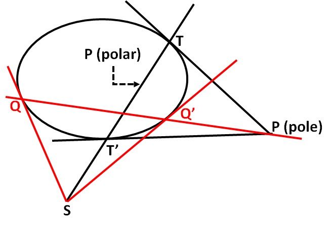
4                                                                         CONTENTS

4 Non-Euclidean Geometry                                                               25

    4.1   Euclid’s Postulate . . . . . . . . . . . . . . . . . . . . . . . . . . . . . 25

    4.2   Saccheri 1667-1733 . . . . . . . . . . . . . . . . . . . . . . . . . . . . 27

    4.3   Lambert 1728-1777 . . . . . . . . . . . . . . . . . . . . . . . . . . . . 29

    4.4   Lobachevskii . . . . . . . . . . . . . . . . . . . . . . . . . . . . . . . . 30

    4.5   Gauss . . . . . . . . . . . . . . . . . . . . . . . . . . . . . . . . . . . 33

    4.6   Bolyai . . . . . . . . . . . . . . . . . . . . . . . . . . . . . . . . . . . 34

    4.7   Riemann . . . . . . . . . . . . . . . . . . . . . . . . . . . . . . . . . . 35

    4.8   Beltrami and Models of Hyperbolic Geometry . . . . . . . . . . . . . 37

    4.9   Klein . . . . . . . . . . . . . . . . . . . . . . . . . . . . . . . . . . . . 38

    4.10 Poincaré . . . . . . . . . . . . . . . . . . . . . . . . . . . . . . . . . . 38

5 State of Geometry by Early 20th Century                                              41

    5.1   Projective Geometry . . . . . . . . . . . . . . . . . . . . . . . . . . . 41

    5.2   Euclidean Geometry . . . . . . . . . . . . . . . . . . . . . . . . . . . 43

    5.3   Non-Euclidean Geometry . . . . . . . . . . . . . . . . . . . . . . . . . 44

6 Space and Geometry                                                                   47

    6.1   Connection of Geometry to the Real World . . . . . . . . . . . . . . . 47

    6.2   Possibilities of Higher Dimensions . . . . . . . . . . . . . . . . . . . . 48

    6.3   Einstein’s Relativity and Minkowski Space-Time . . . . . . . . . . . . 49

    6.4   Is Space Euclidean? . . . . . . . . . . . . . . . . . . . . . . . . . . . . 51

Mark G Watts                                                                   B8428581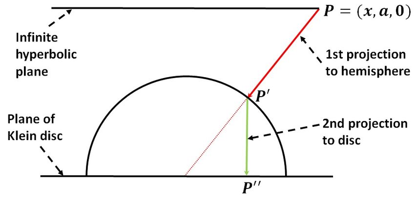
CONTENTS                                                                          5

7 Summary                                                                        53

  7.1   Path 1, Projective Geometry . . . . . . . . . . . . . . . . . . . . . . . 53

  7.2   Path 2, Non-Euclidean Geometry . . . . . . . . . . . . . . . . . . . . 54

  7.3   Subsequent progress . . . . . . . . . . . . . . . . . . . . . . . . . . . 54

A Pole and Polar for a Circle                                                    57

B Models of Hyperbolic Geometry                                                  61

  B.1 Projective, Beltrami Disc, Klein Disc Model . . . . . . . . . . . . . . 61

  B.2 Conformal, Poincaré Disc Model . . . . . . . . . . . . . . . . . . . . . 64

C Michelson Morley Experiment                                                    67

Bibliography                                                                     69

B8428581                                                           Mark G Watts
6              CONTENTS

Mark G Watts     B8428581
Chapter 1

Introduction

The short answer to the question “what was the significance of projective and
non-Euclidean geometry by 1910?” is that projective geometry is now generally
recognised as the single overall geometry with both Euclidean and non-Euclidean
geometries being special cases obtained by projecting in different ways.
Non-Euclidean geometry is considered as valid and self-consistent as is Euclidean
geometry. Further, these two disciplines have brought geometry from almost a
dead subject to one of lively scientific interest and much research.

However the above answer is meaningless without context and the only way to
provide this is to describe some of the developments that led to the above view.

Before we even do that we need to be clear about some terms. We will use the
term Euclidean geometry to describe the geometry as formulated by Euclid in The
Elements [15]. Very specifically this includes what is generally referred to as the
parallel postulate that, given any line and any point not in the line, there is exactly
one line parallel to the given line.

We will use the term non-Euclidean geometry to refer to a geometry which rejects
Euclid’s fifth postulate.

This essay will therefore start with the initial development of geometry as a
science by the ancient Greeks and then trace its path up to 1910. We gloss over
the period from Euclid (c 300 B.C.) to the introduction of perspective by the
Renaissance artists since little of interest to this story happened during this time.
We then follow two parallel paths.

B8428581                                  7                            Mark G Watts
8                                                                1 Introduction

One path, starting with the French mathematicians: Monge, Poncelet, Chasles,
Gergonne, Cauchy, was the development of projective geometry. This was initially
built on the perspective work of the Renaissance artists and all described in a
descriptive manner much the same as the the way that Euclid developed geometry
in The Elements [15] and was often called descriptive geometry. It was further
developed through an algebraic approach by Möbius, Plücker and Cayley until
Cayley was able to state “Metrical [Euclidean] geometry is thus a part of
descriptive [projective] geometry and descriptive geometry is all geometry” [10,
p.592].

The other path started with numerous attempts to prove Euclid’s fifth postulate
and then, through the work of Saccheri, Lambert, Gauss, Bolyai (father and son)
and Lobachevskii, led to the development of non-Euclidean geometry a discipline
just as valid and self-consistent as Euclidean geometry. This was further extended
through the work of Beltrami, Riemann, Poincaré and others until Klein built on
the work of Cayley, above, and showed that non-Euclidean geometry could also be
shown to be a branch of projective geometry.

Thus all branches of geometry were united as part of projective geometry.

This essay discusses the evolution of these two branches in more detail before
discussing the way that geometry is viewed in 1910. This view includes the
axiomatic approach coupled with the duality theories where points and lines are
seen as completely interchangeable as long as the words describing connections are
changed. It also includes an approach to geometry through group theory.

A further, important, aspect of the way geometry is viewed is that it has become a
very active field of research and study whereas at the beginning of the nineteenth
century it was largely regarded as a dead subject in which everything that could
be said about it had already been said.

We also discuss the connection between geometry and the space in which we live.
Is space curved or flat? However, although Einstein’s theory of Special Relativity

Mark G Watts                                                              B8428581
1 Introduction                                                                      9

and Minkowski’s theory of Space-Time show specific examples where space may
not be truly Euclidean on a local scale, there is still no indication whether our
overall universe is Euclidean or non-Euclidean, nor are we likely to ever be able to
find out.

B8428581                                                            Mark G Watts
10             1 Introduction

Mark G Watts         B8428581
Chapter 2

Geometry to End 18th Century

2.1        Greek Geometry

The geometry that is usually taught in high schools is essentially unchanged from
that developed by the Greeks.

Ancient civilisations before the Greeks, especially the Babylonians and Egyptians,
were already using a form of geometry. For example the Egyptians knew the
properties of some Pythagorean triangles so that they could construct right angles
using lengths of wood or rope. The accuracy with which this was done can be seen
in the incredible precision of the pyramids constructed more than 4,500 years ago.
Precise though this was it was essentially a basic construction tool rather than an
academic exercise.

The first attempt to develop geometry into an academic discipline started with
Thales of Miletus (c 625-547 B.C.). In the words of George Allman [2, p.7], he
“introduced abstract geometry, the object of which is to establish precise relations
between the different parts of a figure, so that some of them could be found by
means of others in a manner strictly rigorous”.

This geometry was further developed by many other Greek philosophers and
mathematicians including Pythagoras, Plato and Eudoxus until Euclid formalised,
extended and compiled all this body of knowledge circa 300 B.C. in The
                    1
Elements, [15]          .
   1
       Halsted gives a fascinating account of the way in which The Elements came, via Islamic schol-
ars, to be eventually published in the West.

B8428581                                          11                             Mark G Watts
12 2 Geometry to End 18th Century
Other Geek mathematicians, especially Apollonius of Perga (born c 230 B.C.) and
Archimedes (c 287-212 B.C.), further elaborated this work. Apollonius produced
his Treatise on Conic Sections [4], quoted by the French mathematician Chasles as
containing “The most interesting properties of the conics”.
Among the many results that Archimedes was able to prove we single out his
remarkable determination of upper and lower bounds on the ratio of a circle’s
circumference to its diameter, π, by an iterative method that can theoretically be
continued to any degree of precision. In fact there was a very natural limit due to
the need to perform all the calculations by hand and without the benefit of
modern mathematical notation nor of a positional number system. Nevertheless
Archimedes developed the following result : “The ratio of the circumference of any
circle to its diameter is less than 3 71 and greater than 3 10
71
” [5, p.93], which gives π
to significantly better precision than one part in one thousand..
2.2 Early ideas of Perspective and Projection
Ideas of projection were developed as the Greeks tried to map the known world.
Eratosthenes (c. 275–195 B.C.) is well known for calculating the radius of the
earth by measurements of the shadow projected by a vertical pole at different
latitudes. Later Claudius Ptolemy (c. 90–168) introduced perspective projection
into his maps. Mapmaking continued to evolve and reached a golden period in the
16th and 17th centuries with the work of the Flemish cartographers of whom
Mercator is perhaps the best known. The Mercator projection that he used in his
“... The book that monkish Europe could no longer understand was then taught in Arabic by
Saracen and Moor in the Universities of Bagdad and Cordova.
“To bring the light, after weary, stupid centuries, to western Christendom, an Englishman, Adel-
hard of Bath, journeys, to learn Arabic, through Asia Minor, through Egypt, back to Spain.
Disguised as a Mohammedan student, he got into Cordova about 1120, obtained a Moorish copy
of Euclid’s Elements, and made a translation from the Arabic into Latin” [8, Translator’s Intro-
duction, p.1] .
Mark G Watts B84285812.2 Early ideas of Perspective and Projection 13
1569 world map is a cylindrical projection such as one would obtain by wrapping a
cylinder of paper around the earth and projecting from the axis of the earth onto
the cylinder which is then unrolled into a flat piece of paper.
In parallel with this progress in cartography, artists were exploring ideas of
perspective (from perspico — I observe) to produce more realistic paintings. This
started in the early 15th century with Philippo Brunelleschi, was further developed
by Piero della Francesca about 1470 and fully developed by Dürer into a
mathematical theory of perspective.
A simplified form of this is shown in Figure 2.1 where we imagine viewing a
horizontal scene, the plane (x, y, 0), through an eye placed at C = (0, YC , ZC ).
This forms an image in the plane (x, 0, z) which becomes the artists canvas. It was
through use of such a mechanism that artists were able to convey a realistic
representation of perspective. Some properties of this construction can be readily
proved: points and straight lines in the scene are transformed into points and
straight lines in the canvas. Parallel lines in the scene all meet along a line, the
vanishing line, in the canvas, this is a line in the canvas at the same height as the
eye, (x, 0, ZC ). It is the line to which all points at infinity in the scene are mapped.
This theory of perspective was instrumental in rendering paintings more lifelike
and realistic. Similarly projection was essential for producing maps of the world.
2
But these were not considered as different forms of geometry so essentially the
geometry of the ancient Greeks remained the definitive form.
2
For example Ruskin’s book Elements of Perspective[46], a book aimed at artists, is subtitled
Intended to be read in connexion with the first three books of Euclid.
B8428581 Mark G Watts14 2 Geometry to End 18th Century Figure 2.1: Illustrating the theory of perspective developed by Dürer. The red line shows how the point, P, in the scene is transformed into P’ in the canvas Mark G Watts B8428581
Chapter 3

Projective Geometry

3.1    Monge and the Start of Projective Geometry

Much of the early work in modern projective geometry started in France
immediately after the revolution. This was partly because the new republic needed
geometers to design forts and other weapons of warfare.

Monge [34] started down essentially this line and was soon a professor, teaching his
methods to military students. He developed an approach known as descriptive
geometry whereby a three dimensional object is represented by its projections onto
orthogonal planes and properties worked out by considering each plane separately.
This descriptive geometry helped to better visualise geometric objects and could
greatly simplify proofs and enable less able students to develop ideas in three
dimensional geometry.

As projective geometry developed following Monge, there were many claims and
counter claims about who made the major contribution. We do not attempt here
to follow every development or to postulate on priority. We will certainly not
mention all the actors. However we believe it is instructive to follow the
development of two main themes, both integral to projective geometry:- duality
and cross ratio. These were both being developed at the same time and interact
with each other so there is some overlap in this approach but the two themes are
both central to an understanding of the status of geometry by 1910.

B8428581                                 15                         Mark G Watts
16 3 Projective Geometry
3.2 Duality
3.2.1 Poncelet
In 1822 Poncelet published his memoire on projective geometry, [44]. In it he
develops projective geometry as a separate mathematical discipline. His concept of
projection is similar to that of the artists outlined above, see Figure 2.1, but the
scene and canvas are both in the same plane, as is the eye or projection point.
Poncelet uses projection from a single point to prove many theorems for conics
which are relatively easy to prove in the special case of a circle. He proves the
theorem for a circle then argues that projection about a suitable point can
transform any conic into a circle while transforming individual points and straight
lines into points and straight lines so many theorems can be simply extended from
3
a circle to a general conic. As an example Poncelet proves a duality between
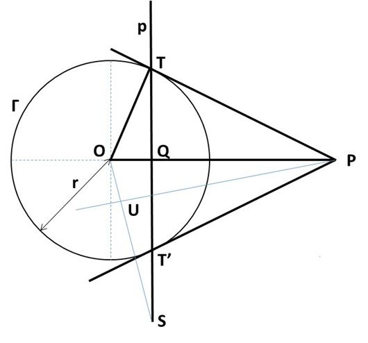
’pole’ and ’polar’ which is illustrated here for an ellipse, Figure 3.1.
Figure 3.1: Illustrating the duality of pole and polar for an ellipse
For any ellipse we choose a point outside the ellipse and call this point, P , a pole.
Construct two tangents from P to touch the ellipse at points T and T 0 . The line
3
This is especially true of theorems involving multiple points in a straight line or multiple lines
intersecting at a single point. It does not apply to any theorems concerning the magnitude of a
distance or an angle
Mark G Watts B84285813.2 Duality 17 T T 0 when extended in both directions is called the polar, p. Now chose any point S on p outside the ellipse, call it a new pole and create a new polar, QQ0 , by constructing the tangents SQ and SQ0 . QQ0 will pass through the original pole, P . Thus there is a duality between pole and polar. This is proved for the circle in Appendix A and can then be extended to all ellipses with the pole outside the ellipse by the simple projection defined above. Extension to other conics and to cases where the pole is inside the conic, or otherwise situated such that it is impossible to construct two real tangents to the conic, are dealt with by Poncelet as he introduces concepts such as ideal chords and his principle of continuity. This is significantly more complicated, maybe even vague, and its justification is still open to some controversy. A book such as Poncelet’s required approval from the French Académie Royale des Sciences and Poncelet has included the report which was prepared by Poisson, Arago and Cauchy. Cauchy chaired the commission and was the most eminent mathematician of the three reviewers (probably the most eminent in France) so we can assume that this mainly expresses his ideas. While the report recommends publication, it does express concern with parts and Cauchy encourages a more algebraic approach including using complex numbers as a way of removing the difficulties with ideal chords and the principle of continuity. Thus Cauchy started to move projective geometry towards a more algebraic approach and may even have anticipated the later work of Plücker and Cayley. 3.2.2 Gergonne Gergonne [19] further extended Poncelet’s concepts to demonstrate that a complete duality exists between points and lines provided that the words used to denote connections — intersect, lie on, cross, meet etc — are adjusted accordingly. He cleverly laid out his results in two columns, one referring to lines connecting points and the other referring to points as the intersection of lines. In this way he was able to (almost) point out the complete duality between points and lines. This B8428581 Mark G Watts
18                                                        3 Projective Geometry

is a much deeper insight than that between pole and polar and later became the
basis of the modern axiomatic approach to projective geometry.

The word “almost” was introduced above because Gergonnes work suffered from
two flaws. The first was quickly rectified by Gergonne himself but the second
required the algebraic approach of Plücker to resolve.

When we consider the dual of a curve we must consider the pole and polar. Thus if
a curve has n tangents from a given point, the pole, its dual will cross the resulting
polar at n points. Gergonne introduced the terms degree and class defined as
follows. The degree of the curve is the maximum number of points at which it is
intersected by a straight line. The class of the curve is the maximum number of
tangents to the curve from a fixed point.

For any curve of degree n the class equals n(n − 1). Conics are of degree 2 so also
of class 2.

Gergonne’s first flaw was that he did not originally distinguish degree from class.
He used the same term, order, for both since he was clearly thinking in terms of
conics where degree and class are both equal to 2. This was quickly corrected
simply by introducing the terms degree and class. The second flaw was more
serious and again it only showed up for curves of degree higher than 2.

3.2.3    Plücker

One of the beauties of duality is that if it is applied twice to a curve the resultant
curve should be the same as the original. However consider forming the dual of the
cubic, a curve of degree 3 so class 3(3 − 1) = 6. The class is the maximum number
of tangents from a fixed point so, when we form the dual, this becomes the
maximum number of points in which the curve is intersected by a straight line.
Therefore the degree of the dual should be 6. Worse follows! The class of the dual
should now be 6.5 = 30. If we now form the dual of this dual its degree should
therefore be 6(6 − 1) = 30. We have now applied duality twice to a curve of degree

Mark G Watts                                                                B8428581
3.2 Duality                                                                           19

3 and obtained, instead of the original curve, a curve of degree 30!

This anomaly was resolved by Plücker [38] by showing that multiple points and
cusps have to be treated especially carefully when passing over to the dual image.
Multiple points and cusps are called singular points. The dual of a double point
(point where the curve crosses itself) is a double tangent (line which touches the
curve at two points). The dual of a cusp is a point of inflection. Plücker showed
that the dual of a curve of degree n with d double points and c cusps is a curve of
degree n(n − 1) − 2d − 3c. With this correction the dual of the dual of a cubic is
again a cubic. The same is true for higher degree curves.

Salmon wrote two excellent textbooks in 1848 and 1852 which formalise and
combine all this earlier work, and more, using an algebraic approach with
homogeneous coordinates throughout. One deals primarily with conic sections [49]
and the other with curves of higher degree, the higher plane curves [50].

3.2.4   Möbius

Whereas Monge, Poncelet, Gegonne and other, mainly French, mathematicians
had used a descriptive approach to projective geometry, Plücker used an algebraic
approach based on the equations of the curves. This approach was already
advocated by Cauchy in his review of Poncelet’s memoire [44] but it was first
taken up seriously by Möbius. He introduced a concept called barycentric
coordinates, which he later simplified to projective, or homogeneous, coordinates,
where each point in a plane was identified by three coordinates rather than the
usual two — only the ratios mattered. This enabled him to identify the point at
infinity in a natural way and not as some limiting process. The point at infinity
therefore became a specific point in the projective plane so statements about lines
and points became simpler and more symmetric. For example any two points
define a line, any two lines meet in a single point. We no longer need to make an
exception in the case of parallel lines because their meeting point is the point at
infinity which has become a perfectly valid point.

B8428581                                                               Mark G Watts
20                                                      3 Projective Geometry

Homogeneous coordinates are defined as follows. Consider the equation of a curve
in a plane. This will be a function of powers of x and y. Replace each instance of x
by x/z and each instance of y by y/z and multiply through to remove inverse
powers of z. The result will be a homogeneous equation in the three variables x, y
and z. As an example consider the general quadratic equation

                         ax2 + by 2 + cxy + dx + ey + 1 = 0

Introducing homogenous coordinates this becomes the homogeneous equation

                       ax2 + by 2 + cxy + dxz + eyz + z 2 = 0

3.3     Cross Ratio

3.3.1   Geometrical Invariants

Veblen and Young [53, §1] start their book on projective geometry with the
statement

“Geometry deals with the properties of figures in space. Every such figure is made
up of various elements (points, lines, curves, planes, surfaces etc.), and these
elements bear certain relations to each other (a point lies on a line, a line passes
through a point, two planes intersect etc.). The propositions stating these
properties are logically interdependent, and it is the object of geometry to discover
such propositions and to exhibit their logical interdependence.”

Some of the properties Veblen and Young refer to are invariants:- they remain
constant under certain transformations. In the two dimensional geometry of Euclid
the possible transformations of the plane are rotation about a fixed point and
translation. Under these transformations points are mapped to points and straight
lines are mapped to straight lines. Further, Euclidean distance, defined by
applying Pythagoras’ theorem, is conserved. Because distance is conserved we can
draw identical triangles in both the un-transformed and transformed systems so
that angles must also be conserved.

Mark G Watts                                                                B8428581
3.3 Cross Ratio 21
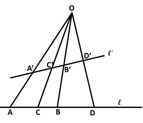
In projective geometry we define a perspectivity as a single projection about a
given point as shown in Figure 3.2. A projectivity is then defined as the product of
one or more perspectivities.
Figure 3.2: Illustrating a perspective transformation or perspectivity. Points
0 0 0 0 0
A, C, B, D on line l are mapped to A , C , B , D on line l via projection in O.
A projectivity will send straight lines to distinct straight lines and points to
distinct points. It will retain the order of the points on a line in the sense that if C
is between A and B then C 0 will be between A0 and B 0 . However it will not
preserve lengths or angles. Lengths and angles are not invariants in projective
geometry.
3.3.2 Cross Ratio Defined
A further conserved property in projective geometry is the cross ratio. We will
introduce this by first defining the harmonic ratio, following Poncelet [44, p.12]
B8428581 Mark G Watts22 3 Projective Geometry
4
Referring to Figure 3.2 we say that C and D cut the line AB harmonically if
AC AD
=−
BC BD
and it also follows that A and B cut the line CD harmonically. A little
rearrangement gives
2 1 1
= +
CD AD BD
So that CD is the harmonic mean of AD and BD.
Still referring to Figure 3.2 we define the anharmonic ratio, or cross ratio, of the 4
points A, C, B, D as
AC/BC AC × BD
(A, B; C, D) = =
AD/BD AD × BC
So that the cross ratio equals −1 if C and D cut the line AB harmonically. This is
the reason the cross ratio was originally called the anharmonic ratio: it measures
the deviation from a harmonic arrangement of four points on a line.
It is easily proven that any perspectivity preserves the cross ratio of any four
distinct points on a line. Therefore any projectivity, being the product of one or
more perspectivities, will also preserve this ratio.
Poncelet states that Pappus of Alexandria was already aware of some properties of
cross ratio but attributes to Brianchon (1807) the proof that cross ratio is
invariant under a perspectivity.
3.3.3 Chasles and Cross Ratios Defined by Angles
Chasles [11, p.11] showed that we can also define cross ratio in terms of the angles
subtended at the point of perspectivity. Thus, still referring to Figure 3.2, he
4
I have changed the terminology slightly since Poncelet appears to refer to the length of the
line from A to C (to the right of A) as CA. I have used AC for this length to be consistent with
other authors, however the result is unchanged since all the negative signs appear in pairs. He
does, however, appear to have missed a negative sign, I believe because he is thinking of a different
arrangement of points from that shown in his Figure [44, Fig. 2], which is essentially the same as
Figure 3.2, above.
Mark G Watts B84285813.3 Cross Ratio 23
5
proved
sin(AOC) sin(BOC) AC BC
÷ = ÷
sin(AOD) sin(BOD) AD BD
This equation immediately proves that cross ratio is preserved for all projections
about a point onto any straight line. It also shows that cross ratio of angles is
preserved as the point of projection is moved, with the four points held constant
on a line. Thus this relation is another example of duality.
3.3.4 Cayley and the Absolute, Link to Euclidean Geometry
Projective geometry is normally described as non-metrical because distances and
angles are not preserved under projection. However Cayley [10] argued that cross
ratio can be used to define a measure of length if two of the points are fixed. The
two points are the points of intersection with a certain conic called the Absolute.
“This absolute configuration must clearly be a curve which every straight line cuts
in two points, real or imaginary, and to which two tangents can be drawn from
every point: i.e. it must be a conic. The absolute in the plane is therefore a fixed
conic, ... in the geometry of Euclid the absolute must be a degenerate conic
consisting of a pair of points, viz. the circular points at infinity” [17, p.157] [51].
With this definition of the absolute Cayley was able to state [10, p.592]
“Metrical [Euclidean] geometry is thus part of descriptive [projective] geometry
and descriptive geometry is all geometry”.
Thus Cayley had shown that Euclidean geometry was a special case of projective
geometry. As we discuss later Klein then expanded on this to show that
non-Euclidean geometry is also a special case of projective geometry. and
produced what is know referred to as the Cayley-Klein metric.
5
Chasles uses lower case symbols for points and upper case for lines. I have changed this for
consistency
B8428581 Mark G Watts24 3 Projective Geometry Mark G Watts B8428581
Chapter 4

Non-Euclidean Geometry

4.1    Euclid’s Postulate

Euclid’s The Elements [15] covers thirteen books containing all of the arithmetic
and geometry known by about 300 B.C., for example it contains his famous
number theory proof that there are infinitely many prime numbers (Book IX,
Proposition 20).

However the majority concerns geometry and it starts in Book 1 with definitions,
postulates and common notations.

We will not quote all 23 definitions but the last is of particular importance to us
“parallel straight lines are straight lines which, being in the same plane and being
produced indefinitely in both directions, do not meet one another in either
direction”.

The common notations are 5 supposedly self evident truths such as “Things which
are equal to the same thing are also equal to one another”.

There are 5 postulates which are quoted in full below:

  1. To draw a line from any point to any point

  2. To produce a finite straight line continuously in a straight line.

  3. To describe a circle with any centre and distance.

  4. That all right angles are equal to one another.

B8428581                                 25                         Mark G Watts
26                                                            4 Non-Euclidean Geometry

     5. If a straight line falling on two straight lines make the interior angles on the
           same side less than two right angles, the two straight lines, if produced
           indefinitely, meet on that side on which the angles are less than two right
           angles.

Postulates 1 and 2 would today be written something like

     1. Any two non-coincident points uniquely define a straight line.

     2. A straight line can be continued indefinitely without intersecting itself.

Postulate number 5, the parallel postulate, has been the subject of much debate
ever since The Elements were first written. There is a strong suggestion that
Euclid was not sure of the validity of this postulate since he placed it last and
ordered his propositions (theorems) such that early ones did not depend on the
parallel postulate. It is only in proposition 29 that the parallel postulate is first
used. The parallel postulate has been stated in many different, but essentially
equivalent, ways. One form is what is generally known as Playfair’s axiom: “given
any line and a point in the same plane but not on the line, there is exactly one line
through the point which is parallel to the given line” 6 .

There are many consequences of the parallel postulate which are often taken for
granted, such as that the interior angles of any triangle sum to two right angles or
180◦ . Also that triangles can be scaled and still retain the same angles — similar
triangles.

Many mathematicians, starting with the ancient Greeks:- Diodorus, Proclus and
Ptolemy; through the Persians to the great French mathematician, Legendre
(1752-1833), have tried to prove the parallel postulate from the first 4 postulates
but to no avail. A good summary of these accounts is given in Euclid’s The
Elements, Book 1, Note on Postulate 5 [15, pp.202-220]. All these attempts to
     6
         In fact Playfair writes this as “That two straight lines which cut one another cannot be both
parallel to the same straight line” and attributes this statement to Ludlam [37, p.291] .

Mark G Watts                                                                              B8428581
4.2 Saccheri 1667-1733 27
prove the parallel postulate show how deep seated was the common belief in its
truth.
4.2 Saccheri 1667-1733
Saccheri [48] took a somewhat different approach, aiming for a proof by
contradiction, reductio ad absurdum. He was also totally convinced of the truth of
the parallel postulate so he set out to develop a self-consistent geometry based on
the first four postulates but denying the fifth. The intent was that he would at
some point find an inconsistency which would automatically justify the parallel
postulate.
In 1733 he published his Euclides ab omni naevo vindicatus, [Euclid freed of every
fleck ], subtitled a geometric endeavor in which are established the foundation
principles of universal geometry.
Saccheri starts by assuming the first 4 postulates and refuting the fifth. He then
develops very simple geometrical arguments based on the simple construction,
Figure 4.1, of a straight line, AB, on which he raises 2 equal perpendiculars, AC
and BD, and joins CD. Use of the parallel postulate would show this to be a
rectangle so CD = AB but Saccheri does not assume this. Instead he shows that
the angles at C and D must be equal and distinguishes 3 cases 7 :
har: right angle, C = D = π/2, CD = AB
hao: obtuse angle, C = D > π/2, CD < AB
haa: acute angle, C = D < π/2, CD > AB
He then goes on to show that case har implies that all triangles will have angles
summing to π, hao implies they will always sum to values > π and haa that they
will always be < π. He is then able to show that case hao produces a contradiction
7
I have used the abbreviations of the names Saccheri gives to each of these hypotheses, respec-
tively: hypothesim anguli recti, hypothesim anguli obtusi, hypothesim anguli acuti
B8428581 Mark G Watts28 4 Non-Euclidean Geometry Figure 4.1: The quadrilaterals constructed by Saccheri (left) and Lambert (right) with the right angles marked. Saccheri inserts the line M H where M and H are the mid points of AB and CD respectively and then proves that angles AM H and CHM are right angles so Lambert’s quadrilateral is exactly the same as the right half of Saccheri’s quadrilateral and, erroneously, proves that haa also has a contradiction. That he gets to this latter result despite all the good earlier work is probably due to his total belief in the parallel postulate. He needed to prove it true so was somewhat blind to the error in his arguments. This is somewhat equivalent to the well known concept of “flinching” in experimental work where the experimentalist knows the result he expects and keeps measuring until he arrives at it. Saccheri talks of wanting to tear out by its very roots “the hostile hypothesis of acute angle”. Halsted comments [21, p.101] “Saccheri was always fighting against the heretical results of his own logic on behalf of what he considered God’s truth.” In fact Saccheri had gone a long way towards discovering hyperbolic geometry, over 100 years before Lobachevskii’s famous paper which will be described later. Mark G Watts B8428581
4.3 Lambert 1728-1777                                                               29

4.3    Lambert 1728-1777

It is not clear how much Lambert knew of Saccheri’s work. He starts from a
different position with a diagramme similar to that later used by Lobachevskii, see
Figure 4.2 but then in section 39 [14, p.180] introduces a quadrilateral very similar
to that used by Saccheri Figure 4.1 and lists 3 hypotheses, he will develop, namely

    Hypothesis 1. BDC = 90 degrees
    Hypothesis 2. BDC > 90 degrees
    Hypothesis 3. BDC < 90 degrees

So this part of his work is very similar to Saccheri’s.

He shows, as had Saccheri, that hypothesis 2 leads to a contradiction if we retain
Euclid’s second postulate that lines can be continued indefinitely without meeting.
He failed to prove that his hypothesis 3 (acute angle) led to a contradiction and
thereby developed a new self-consistent geometry, now known as hyperbolic
geometry.

Lambert also showed that a self-consistent geometry can be developed based on
the hypothesis of an obtuse angle, hypothesis 2, if he relaxed Euclid’s second
postulate and allowed the radius to be imaginary. This is similar to the geometry
on the surface of a sphere and is now called spherical geometry.

Lambert was able to prove that in both hypotheses 2 and 3 the angles of a triangle
did not sum to two right angles. If the angles are denoted by α, β and γ he proved
that α + β + γ − 2π is positive for hypothesis 2 (obtuse angle) and negative for
hypothesis 3 (acute angle) and, in both cases, is proportional to the area of the
triangle. This then led him to the conclusion that there must be an absolute
measure of length since there is obviously an absolute measure of angle.

It appears that Lambert was not satisfied with this work, as he had set out, and
failed, to find an inconsistency which would validate Euclid’s fifth postulate, and
he did not publish it in his lifetime. Frankland [16] suggests that the work was

B8428581                                                            Mark G Watts
30 4 Non-Euclidean Geometry
completed in 1766. It was published posthumously in 1786 as “Die Theorie der
8
Parallellinien” and was then republished by Engel and Stäckel [14] in 1895
Lambert makes the following comment on his failure to disprove his 3rd
hypothesis [16, p.25]:
“This consequence possesses a charm which makes one desire that the Third
Hypothesis be indeed true!
“Yet on the whole I would not wish it true, notwithstanding this advantage (of an
absolute standard length), since innumerable difficulties would be involved
therewith. Our trigonometric tables would become immeasurably vast; the
similitude and proportionality of geometrical figures would wholly disappear, so
that no figure can be represented except in its actual size; astronomy would be
harassed.”
4.4 Lobachevskii
Lobachevskii is today generally regarded, along with Gauss and Bolyai, as being
the founder of hyperbolic geometry. His translator, Halsted, tells us that [29, p.8]
“the first public expression ... dates back to a discourse at Kasan on February 12,
1826”. His paper was then published, in sections, in Russian, in the Kasan
Messenger, between 1829 and 1830 [20, p.120], and totally ignored outside of
Russia. Lobachevskii then translated this into German and republished it in a
German journal in 1840 and this is the version that is now most known.
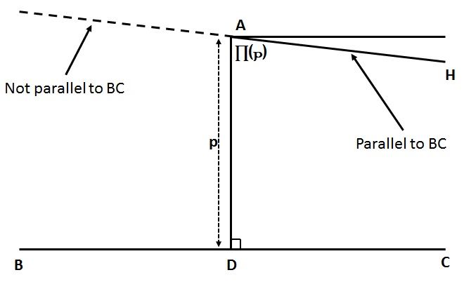
Lobachevskii’s starting point is his definition of parallel and angle of parallelism,
Figure 4.2. He splits lines through A into 2 classes, those cutting BC and those not
8
Despite an extensive literature search I have been unable to find an English translation of
Lambert’s paper. This is a great shame since it was originally written in 1766, fully 60 years
before Lobachevskii first started to share his views on hyperbolic geometry, and therefore should
be considered the first publication on non-Euclidean geometry.
Mark G Watts B84285814.4 Lobachevskii 31
9
cutting, and calls the boundary line, AH, between the 2 classes the parallel line.
The angle of parallelism, Π(p), is defined as the angle between AH and AD, the
perpendicular to BC. Π(p) is a function of p, the perpendicular distance of A from
BC. If Π(p) = π/2 we clearly have Euclidean geometry. Lobachevskii focuses on
the case where Π(p) < π/2.
It is important to notice that, if we define line AH to be parallel to BC, then the
continuation of HA beyond A will not, in general, be parallel to BC.
Figure 4.2: Definition of parallel and the angle of parallelism, Π(p)
He defines a horocycle as a curve such that the perpendicular bisectors of all its
chords are parallel, see Figure 4.3. Euclidean geometry holds on a horocycle so he
is able to show that the length of a horocycle between two parallel lines reduces as
e−x where x is the distance along an axis between the two horocycles. See
Figure 4.4 which gives s0 = se−x .
From the relation s0 = se−x , Lobachevskii is able to derive the relationship
1
tan Π(x) = e−x (4.1)
2
9
Lobachevskii makes a distinction between “parallel” and “not cutting” which had not been
made before. In fact these terms were almost used interchangeably in Euclidean geometry.
B8428581 Mark G Watts32 4 Non-Euclidean Geometry
Figure 4.3: Illustrating the definition of a horocycle. EF , GH and JK are parallel
in the definition of Lobachevskii
Figure 4.4: Illustrating reduction of a horocycle between parallel lines, s0 = se−x
And he was then able to develop relationships between the angles of a triangle,
10
valid in hyperbolic geometry , which reduce, for small triangles, to the sine rule,
the cosine rule and the condition that the angles of a triangle sum to 180◦ .
He also shows that his equations reduce to identities pertaining to spherical
√
triangles if lengths are all multiplied by −1 11 . This is similar to the result
obtained by Lambert.
Lobachevskii’s fundamental relationship which was shown as Equation 4.1 directly
10
These relationships include Π(x), the angle of parallelism, so are dependent on the size of the
triangle. This explains Lambert’s concern over the size of trigonometric tables, see Section 4.3
11
This will replace the hyperbolic functions by trigonometrical functions.
Mark G Watts B84285814.5 Gauss 33
relates an angle to a distance and so this again shows that hyperbolic geometry
directly implies an absolute measure of distance.
4.5 Gauss
Gauss is now credited, along with Lobachevskii and Jànos Bolyai, with the
discovery of non-Euclidean geometry although he published very little during his
lifetime. His unpublished work, discovered after his death, show that his ideas
were very well developed.
While he was working as a geodesist, directing the triangulation survey of
Hannover, Gauss developed a measure of the curvature of a plane surface. He
1
defined Gaussian curvature as r1 r2
where r1 and r2 are the greatest and least radii
of curvature at a point on a surface. In this he is relating his curved surface to a
third, orthogonal, dimension since he was actually interested in the curvature of
points on the surface of the earth.
From Gauss’s definition of curvature we see that the curvature on both the inside
and outside surface of a sphere must be positive, that on the surface of a cylinder
must be zero. Negative curvature will be obtained near a saddle point where the
curvature in one plane is positive and in the orthogonal plane negative.
To derive his expression for curvature, Gauss assumes that the position on a
12
curved surface, (x, y, z) can be expressed as a function of two variables, u, v and
writes a line element in the form
√
ds = Edu2 + 2F dudv + Gdv 2
where E, F and G are sums of products of the partial derivatives of the x, y and z
coordinates, with u and v. He then writes the curvature, k, as an expression
involving just E, F, G and their first and second derivatives with respect to u and
12
Gauss uses p, q but I use u, v here for consistency with later authors such as Beltrami, Sec-
tion 4.8.
B8428581 Mark G Watts34 4 Non-Euclidean Geometry
v. [18, p.20]
“The analysis developed in the preceding article thus shows that for finding the
measure of curvature there is no need for finite formulae, which express the
coordinates x, y, z as functions of the indeterminates u, v; but that the general
expression for the magnitude of any linear element is sufficient.” — As long as you
can find E, F, G as functions of u and v you can calculate the curvature.
Significantly, Gauss had shown that, although he had introduced a third
dimension, the equation for the curvature does not involve this third dimension.
This was later expanded by Riemann who developed a general theory of curvature
of manifolds.
Gauss showed that the curvature of a triangle on a curved surface can be obtained
simply by summing its angles “The excess of the sum of the angles of a triangle
formed by shortest lines over two right angles is equal to the total curvature of the
13
triangle.” [18, p.48] .
He illustrated this theory via direct measurements between 3 hilltops in Germany,
one side of was over 100 km, where the excess in the sum of the angles over two
right angles is 14.85 seconds of arc.
4.6 Bolyai
Jànos Bolyai developed a theory of parallels [8] independently from, but
remarkably similar to, that of Lobachevskii. It was originally published in 1832 as
an appendix to a joint work with his father, Farkas (Wolfgang) Bolyai. This in
turn contains an appendix to the appendix, written by Farkas, which points out
many of the similarities between his son’s work and that of Lobachevskii. For
example, Bolyai introduces a concept called an L-curve, similar to Lobachevskii’s
13
Naturally this must be normalised for the size of the triangle, Gauss explains how the units
should be chosen to achieve this.
Mark G Watts B84285814.7 Riemann 35 horocycle, and an F-surface, similar to the horosphere, which is a surface of revolution of the L-curve. The useful property of the L-curves (and of horocycles) is that Euclidean geometry holds on them and therefore properties in hyperbolic geometry can be related to trigonometric functions. Since Bolyai’s conclusions are similar to Lobachevskii’s we will not discuss them further here but one significant difference in their approaches is that Lobachevskii uses a descriptive approach, in which he derives theorems in a manner similar to the approach taken by Euclid, whereas Bolyai uses an algebraic approach and develops many of his results through application of calculus. 4.7 Riemann One of Riemann’s most celebrated works in geometry is his Habilitationsvorstrag [45], the lecture with which he defended his doctoral thesis, presented in front of Gauss and a full lecture theatre of academics and students. This paper contains only one equation so he has to express all his profound ideas in words. It develops a totally new approach to geometry based on the concepts of multiply extended quantities and of manifolds. The concept of multiply extended quantities was used to build up the notion of an n dimensional space without having to resort to Cartesian or any other coordinate system. The concept of a manifold described a portion of space which could have a totally different structure, and curvature, from its neighbouring manifolds, except, of course, that the whole of space must be continuous. In this lecture, Riemann developed a theory of a generalised space which could have any curvature but without mentioning hyperbolic geometry. Several of his audience were from the Philosophy department, of which Mathematics was a part, and did not need to be shocked by such outrageous ideas as non-Euclidean geometry. Nevertheless Riemann specifically develops his ideas of non-zero curvature. He considers both positive and negative curvature and points out that B8428581 Mark G Watts
36 4 Non-Euclidean Geometry
geometries with positive curvature can be wrapped around the surface of a type of
sphere and so are finite provided Euclid’s second is also rejected. This became
known as Riemannian or spherical geometry14
He also shows that negative curvature is just as valid as is zero curvature so laying
the foundation for the legitimisation of hyperbolic geometry.
Riemann’s single equation in his Habilitationsvorstrag is an expression relating
curvature to the length of a line element. He starts from, but does not state in this
15
lecture, the assumption that the line element can be written in the form
qX
ds = aij dxi dxj (4.2)
He then states that, if we write α for the curvature, this expression for the line
element becomes
1
qX
ds = α dx2i (4.3)
x2i
P
1+ 4
1
Or, writing r2
for the curvature, α, we obtain in two dimensions
p
dx2 + dy 2
ds = (4.4)
1 + (1/4r2 )(x2 + y 2 )
the form in which it is quoted by Gray [20, p.200].
Helmholtz [22, p.48] explores the validity of the assumptions contained in
Equation 4.2. He makes 4 assumptions:-
14
This is not exactly the same as the geometry of the surface of the earth since geodesics meet
in two points on the earth (e.g. all lines of longitude meet at the North and South poles). This
would also be a violation of Euclid’s first postulate which Riemann retains.
15
Klein [27, p.86] clarifies this by saying “...he only wants to say that there exists an invariant
P
of the ‘form’ aij dxi dxj ; he does not mean to imply that the three-dimensional space necessarily
exists as a curved space in a space of four dimensions.”
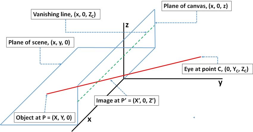
Mark G Watts B84285814.8 Beltrami and Models of Hyperbolic Geometry 37 • Continuity • Rigid bodies can move freely (implies constant curvature) • Free mobility of points • Invariance under rotation (called mondromy by Helmholtz) and then states “it follows from pure analysis that a homogeneous function of the second degree of the magnitudes du, dv, dw exists...” . With this he shows that Equation 4.2 is the simplest general form satisfying his 4 assumptions. Riemann had introduced a new concept in geometry, to quote Gray [20, p.201] “To him, geometry was to do with concepts like length and angle which could be intrinsically defined on a surface or space of some sort. It follows that there are many geometries, one for each kind of surface and each definition of distance...”. Thus Riemann had broadened the whole of geometry and in the process had given his stamp of approval, as the leading mathematician of his generation, to non-Euclidean geometry as a valid geometry. 4.8 Beltrami and Models of Hyperbolic Geometry In two remarkable papers in 1868 [6] [7], Beltrami further developed Riemann’s ideas about curvature and in so doing developed relationships between hyperbolic geometry and models which can be visualised in a Euclidean disc or sphere. Thus he was the first to develop models of hyperbolic geometry. He developed all this in terms of transformations of coordinates so there are no diagrammes to show the nature of the underlying projections. In his first paper, usually referred to as his Saggio [6], essay, he develops the mathematics of what is know known as the Klein disc, see Section B.1. In the second paper [7] he develops several other models including the conformal model which is now referred to as the Poincaré disc, Section B.2. B8428581 Mark G Watts
38                                                  4 Non-Euclidean Geometry

This work was largely ignored at the time of publication and both the above and
other models were later rediscovered or further developed by others and Beltrami’s
name has largely been forgotten as the originator of these models.

They are described in more detail in Appendix B.

4.9    Klein

Klein realised that Cayley’s unification of projective and Euclidean geometries, see
Section 3.3.4, could be further extended to unite non-Euclidean geometry with
projective geometry. This can be done by choosing a different absolute but Klein
proceeds from first principles by first defining how to set up a measure of length,
then defining a scale which is exponential and defining the length as a logarithmic
measure on this scale. Thus he defines the distance between two elements as
                                               z
                                       c log
                                               z0
and interprets z/z 0 as a cross ratio when two other points on the line have been
moved to z = 0 and z = ∞,       i.e. log z = ∓∞.

This works for real one dimensional lines where the line passes through the point
z = 0. In two dimensions Klein simply uses complex lines to describe lengths and
obtains a result similar to that of Cayley.

Kleins use of cross ratio and the Cayley-Klein metric are illustrated in a
diagramme of the Klein disc in Section B.1.

4.10     Poincaré

Poincaré was a true polymath and made significant contributions in many fields of
mathematics, physics, engineering and philosophy. He was able to link supposedly
unconnected fields. Thus his work on what he called fuschian groups [40] led to his

Mark G Watts                                                                 B8428581
4.10 Poincaré 39
independent development of the Poincaré disc model, see Section B.2.
Fuschian groups are a class of elliptic functions (doubly periodic functions) which
are invariant under a group of mappings of the form
az + b
z 7→ , where ad − bc 6= 0 (4.5)
cz + d
This type of bilinear transformation is called a Möbius transformation and
Poincaré realised that it had the following characteristics
• It preserves angles
• It is monogenic (one to one)
• It maps circles into circles
• “Finally [39, p.124], if z1 , z2 , z3 , z4 are four values of z and if t1 , t2 , t3 , t4 are
the corresponding values of t, then
t1 − t2 t4 − t3 z1 − z2 z4 − z3
= ”
t1 − t3 t4 − t2 z1 − z3 z4 − z1
Therefore this was an ideal model of a conformal (angle preserving) mapping. In
particular the last property shows that it preserves cross ratio so it is also a
projective mapping. This then became the basis of Poincaré’s development of the
disc that bears his name. If we set |a/c| = 1 this maps the entire plane into the
open unit circle. Poincaré also showed that depending whether the value of
(a + d)2 is less than, equal to, or greater than 4 this can be a model of spherical,
Euclidean, or hyperbolic geometries respectively.
In the above paper Poincaré focussed on real transformations where a, b, c, d are all
real. In a subsequent paper entitled Memoire on Kleinian Groups [40] he considers
a, b, c, d all complex in Equation 4.5. He shows that the Möbius transformation
that defines this mapping can also be arrived at by an even number of inversions in
the unit disc and finally is able to show a connection between the theory of linear
transformations and non-Euclidean geometry.
B8428581 Mark G Watts40 4 Non-Euclidean Geometry Thus through the work of Klein, Beltrami and Poincaré a total connectivity had been made between projective and non-Euclidean geometries and therefore also Euclidean geometry. ‘ Mark G Watts B8428581
Chapter 5

State of Geometry by Early
20th Century

5.1    Projective Geometry

Although projective geometry is still often taught as an extension of high school
geometry, the formal, axiomatic, approach is now usually favoured by
mathematicians.

A central part of this is duality, based on the concepts introduced by Gergonne but
further developed. No distinction is made between points and lines, or even planes.
They are simply abstract concepts that are connected by certain relationships.
Veblen and Young [53, p.29] call this connectivity on so that points are said to lie
on a line, lines lie on a point etc. They then state:

“Any proposition ... concerning the points and lines of a plane remains valid, if
stated in the on terminology, when the words point and line are interchanged.

“...Any proposition ... concerning the planes and lines through a point remains
valid, if stated in the on terminology, when the words plane and line are
interchanged.”

Another essential feature of projective geometry is the algebraic approach and the
use of homogeneous coordinates where x and y are replaced by x/z and y/z, see
Section 3.2.4. This enables significant simplifications, including:

B8428581                                  41                          Mark G Watts
42                              5 State of Geometry by Early 20th Century

     • The point at infinity appears naturally by setting z = 0, thus the projective
        plane has an extra point. There is now no need to have exceptions to rules as
        in for example any two lines meet at a point unless they are parallel

     • The point at infinity leads to the distinction between ordinary points, where
        z 6= 0, and Ideal points, where z = 0. This definition of Ideal points opens the
        way for the work of Cayley and Klein on unifying projective geometry with
        Euclidean and non-Euclidean geometry

     • Equations of points, lines and planes appear in a more symmetrical form.
        Thus a point can be denoted (a, b, c), meaning x = a, y = b, z = c, and a line
        can be denoted by (ξ, η, ζ) meaning ξx + ηy + ζz = 0. Further the
        requirement that the point is on the line is aξ + bη + cζ = 0 which is also the
        requirement that the line is on the point.

     • Many relationships and transformations, e.g. between points and lines, can
        be expressed via linear algebra and can therefore be written in matrix
        notation.

Modern geometry also began to be stated in terms of group theory through the
work of Sophus Lie but here explained by Poincaré [42, p.9]:

“It is obvious that if we consider a change A, and cause it to be followed by
another change B, we are at liberty to regard the ensemble of the two changes A
followed by B as a single change which may be written A + B and may be called
the resultant change. (It goes without saying that A + B is not necessarily
identical with B + A.) The conclusion is then stated that if the two changes A and
B are displacements, the change A + B also is a displacement. Mathematicians
express this by saying that the ensemble, or aggregate, of displacements is a group.
                                                                  16
If such were not the case there would be no geometry.”

Group theory implies symmetries and invariants. Thus two invariants of Euclidean
 16
      Nowadays we would write B.A where Poincaré writes A + B.

Mark G Watts                                                                 B8428581
You can also read