Survey: Sixty Years of Douglas-Rachford
←
→
Page content transcription
If your browser does not render page correctly, please read the page content below
Survey: Sixty Years of Douglas–Rachford
                                                       Scott B. Lindstrom                           Brailey Sims
arXiv:1809.07181v2 [math.OC] 21 Feb 2019

                                                            CARMA                                     CARMA
                                                     University of Newcastle                   University of Newcastle
                                                                              February 22, 2019

                                           Dedication
                                           This work is dedicated to the memory of Jonathan M. Borwein our greatly missed
                                           friend, mentor, and colleague. His influence on both the topic at hand, as well as his
                                           impact on the present authors personally, cannot be overstated.
                                                                                      Abstract
                                                      The Douglas–Rachford method is a splitting method frequently employed for
                                                 finding zeroes of sums of maximally monotone operators. When the operators in
                                                 question are normal cones operators, the iterated process may be used to solve fea-
                                                 sibility problems of the form: Find x ∈ N
                                                                                          T
                                                                                            k=1 Sk . The success of the method in the
                                                 context of closed, convex, nonempty sets S1 , . . . , SN is well-known and understood
                                                 from a theoretical standpoint. However, its performance in the nonconvex context
                                                 is less understood yet surprisingly impressive. This was particularly compelling to
                                                 Jonathan M. Borwein who, intrigued by Elser, Rankenburg, and Thibault’s success
                                                 in applying the method for solving Sudoku Puzzles began an investigation of his
                                                 own. We survey the current body of literature on the subject, and we summarize its
                                                 history. We especially commemorate Professor Borwein’s celebrated contributions
                                                 to the area.

                                           1    Introduction
                                           In 1996 Heinz Bauschke and Jonathan Borwein broadly classified the commonly ap-
                                           plied projection algorithms for solving convex feasibility problems as falling into four
                                           categories. These were: best approximation theory, discrete models for image re-
                                           construction, continuous models for image reconstruction, and subgradient algorithms
                                           [18]. One such celebrated iterative process has been known by many names in many
                                           contexts and is possibly best known as the Douglas–Rachford method (DR).
                                               DR is frequently used for the more general problem of finding a zero of the sum
                                           of maximally monotone operators, which itself is a generalization of the problem of
                                           minimizing a sum of convex functions. Many volumes could be written on monotone
                                           operator theory, convex optimization, and splitting algorithms specifically, the defini-
                                           tive work being that of Bauschke and Combettes [21]; the story of DR is inextricably
                                           entwined with each of these.

                                                                                          1
More recently, the method has become famous for its surprising success in solving
nonconvex feasibility problems, notwithstanding the lack of theoretical justification.
The recent investigation of these methods in the nonconvex setting has been both moti-
vated by and advanced through experimental application of the algorithms to noncon-
vex problems in a variety of different settings. In many cases impressive performance
has been observed despite having previously been thought of as ill-adapted to projec-
tion algorithms.
The task of choosing what to include in a condensed survey of DR is thus neces-
sarily difficult. We therefore choose to adopt an approach which balances reasonable
brevity with the goal that a reader unfamiliar with DR should be able to at least glean
the following: the basic history of the method, an understanding of the various mo-
tivating contexts in which it has been “discovered,” an appreciation for the diversity
of problems to which it is applied, and a sense of which research topics are currently
being explored.
1.1 Outline
This paper is divided into four sections:
Section 1 In 1.2, we provide preliminaries on Douglas–Rachford and feasibil-
ity. In 1.3, we briefly motivate its history and explain how feasibility
problems are a special case of finding a zero for a sum of maximal
monotone operators, and in 1.4 we explore its use for finding ze-
ros of maximal monotone operator sums, including its connection
with ADMM in 1.4.1. In 1.5, we analyse the ways in which it has
been extended from 2 set feasibility problems to N set feasibility
problems.
Section 2 We consider the role of DR in solving convex feasibility problems.
In 2.1 we catalogue some of the convergence results, and in 2.2 we
mention some of its better known applications.
Section 3 We consider the context of nonconvex feasibility. We first consider
discrete problems in 3.1 and go on to discuss hypersurface problems
in 3.2. In 3.3, we explore some of the possibly nonconvex conver-
gence results which employ notions of regularity and transversality.
In 3.3.3 we describe some of the recent work applying DR for non-
convex minimization problems.
Section 4 Finally we mention two open problems and summarize the current
state of research in the field.
Appendix 5 This appendix provides a more detailed summary of Gabay’s expo-
sition on the connection between DR and ADMM.
21.2 Preliminaries
The method of alternating projections (AP) and the Douglas–Rachford method (DR)
are frequently used to find a feasible point (point in the intersection) of two closed
constraint sets A and B in a Hilbert space H. The feasibility problem is
Find x ∈ A ∩ B. (1)
The projection onto a subset C of H is defined for all x ∈ H by
0
PC (x) := z ∈ C : kx − zk = inf0
kx − z k .
z ∈C
Note that PC is, generically, a set-valued map where values may be empty or contain
more than one point. In the cases of interest to us PC has nonempty values (indeed
throughout PC is nonempty and so C is said to be proximal), and in order to simplify
both notation and implementation, we will work with a selector for PC , that is a map
PC : H → C : x 7→ PC (x) ∈ PC (x), so PC2 = PC .
When C is nonempty, closed, and convex the projection operator PC is uniquely
determined by the variational inequality
(x − PC (x), c − PC (x)) ≤ 0, for all c ∈ C,
and is a firmly nonexpansivemapping; that is for all x, y ∈ H
kPC x − PC yk2 + k(I − PC )x − (I − PC )yk ≤ kx − yk2 .
See, for example, [21, Chapter 4]. When C is a closed subspace it is also a self-adjoint
linear operator [21, Corollary 3.22].
The reflection mapping through the set C is defined by
RC := 2PC − I,
where I is the identity map.
Definition 1.1 (Method of Alternating Projections). For two closed sets A and B and
an initial point x0 ∈ H, the method of alternating projections (AP) generates a sequence
(xn )∞
n=1 as follows:
xn+1 := PB PA xn . (2)
Definition 1.2 (Douglas–Rachford Method). For two closed sets A and B and an initial
point x0 ∈ H, the Douglas–Rachford method (DR) generates a sequence (xn )∞ n=1 as
follows:
1
xn+1 ∈ TA,B (xn ) where TA,B := (I + RB RA ) . (3)
2
DR is often referred to as reflect-reflect-average. Both DR and AP are special cases
of averaged relaxed projection methods. We denote a relaxed projection by
γ
RC (x) := (2 − γ)(PC − Id) + Id, (4)
3for a fixed reflection parameter γ ∈ [0, 2). Observe that when γ = 0, the operator
γ=0
RC = 2PC − Id is the standard reflection employed by DR, and for γ = 1 we obtain
γ γ
the projection, RC = RC1 = PC . For γ ∈ (1, 2) the operator RC can be called an under-
relaxed projection following [71]. Here we are using the terminology in (4). However,
γ γ
the reader is cautioned that in some articles, RC is written as PC , while in others the
role of γ is reversed so that γ = 2 corresponds to a reflection and γ = 0 is the identity:
γ(PC − Id) + Id.
In addition to using relaxed projections as in (4), the averaging step of the Douglas–
Rachford iteration can also be relaxed by choosing an arbitrary point on the interval
between the second reflection and the initial iterate. This can be parametrised by some
λ ∈ (0, 1]. Accordingly we define a λ -averaged relaxed sequence {xn } by,
n n
µ γ
xn := TAλγ ,Bµ x0 := λ (RB ◦ RA ) + (1 − λ )Id x0 . (5)
When λ = γ = µ = 1, this is the sequence generated by alternating projections (2), and
for λ = 1/2 and γ = µ = 0, this is the standard Douglas–Rachford sequence (3). For
γ = µ = 0 and λ = 1, this is the Peaceman-Rachford sequence [125] (see also Lions &
Mercier [117, Algorithm 1]).
We note that the framework introduced here does not cover all possible projection
methods. For example, one may want to vary the parameters γ, µ and λ on every step,
or consider other variations of Douglas–Rachford operators (see [10] for example).
Single steps of the AP and DR methods are illustrated in Figure 1, which originally
appeared in [73].
HA HB HA
HB
B
B RB RA x
x x
TA,B x
PA x PA x PB RA x
PB PA x
RA x
A A
(a) One step of alternating projections (b) One step of Douglas–Rachford method
Figure 1: The operator TA,B .
Definition 1.3. The fixed point set for a mapping T : H → H is Fix T = {x ∈ H | T x = x}
(in the case when T is set-valued Fix T = {x ∈ H | x ∈ T x}.
41.3 History
Projection methods date at least as far back as 1933 when J. von Neumann considered
the method of alternating projections when A and B are affine subsets of H establishing
its norm convergence to PA∩B (x0 ) [138]. In 1965 Bregman showed that in the more
general setting where A and B are closed convex sets AP converges weakly to a point
in A ∩ B [56](see also [18]). In 2002 Hundal [110] provided an example in infinite
dimensions of a hyperplane and closed cone for which AP fails to converge in norm.
However the cone constructed by Hundal is somewhat unnatural. In [51] Borwein,
Sims, and Tam explored the possibility of norm convergence for sets occurring more
naturally in applications.
Sixty years ago the Douglas–Rachford method was introduced, somewhat indi-
rectly, in connection with nonlinear heat flow problems [74]; see [120] for a thorough
treatment of the connection with the form we recognize today. The definitive statement
of the weak convergence result was given by Lions and Mercier in the more general set-
ting of maximal monotone operators [117]. We will first state the problem and result,
and then explain the connection. The problem is
Find x such that 0 ∈ (A + B)x. (6)
Let the resolvent for a set-valued mapping F be defined by JFλ := (Id + λ F)−1 with
λ > 0. The classical result is as follows.
Theorem 1.4 (Lions & Mercier [117]). Assume that A, B are maximal monotone op-
erators with A + B also maximal monotone, then for
TA,B : X → X : x 7→ JBλ (2JAλ − I)x + (I − JAλ )x (7)
the sequence given by xn+1 = TA,B xn converges weakly to some v ∈ H as n → ∞ such
that JAλ v is a zero of A + B.
The normal cone to a set C at x ∈ C is NC (x) = {y ∈ H : (y, c − x) ≤ 0 for all c ∈ C}.
The normal cone operator associated to C is
NC (x), when x ∈ C
NC : H → H : x 7→ (8)
0,
/ when x ∈ / C.
See, for example, [21, Definition 6.37]. One may think of the feasibility problem (1)
as a special case of the optimization problem
Find x ∈ argmin {ιA + ιB } (9)
where the indicator function ιC for a set C is defined by
(
0 if x ∈ C
ιC : H → R∞ by ιC : x 7→ . (10)
∞ otherwise
Whenever A and B are closed and convex, ιA and ιB are lower semicontinuous and
convex, and their subdifferential operators ∂ ιA = NA and ∂ ιB = NB are maximal mono-
tone. In this case, under satisfactory constraint qualifications on A, B to guarantee the
5sum rule for subdifferentials ∂ (ιA + ιB ) = ∂ ιA + ∂ ιB (see [21, Corollary 16.38]), the
problem (9) reduces to
Find x such that 0 ∈ (∂ ιA + ∂ ιB ) (x) = (NA + NB ) (x) (11)
which we recognize as (6). Seen through this lens, two set convex feasibility is a spe-
cial case of an extremely common problem in convex optimization: that of minimizing
a sum of two convex functions f + g where A = ∂ f and B = ∂ g. This illuminates
its close relationship to many other proximal iteration methods, including the various
augmented Lagrangian techniques with which it is often studied in tandem (see sub-
section 1.4.1).
Where A = NA and B = NB are the normal cone operators for closed convex sets A
and B, then the resolvents JAλ , JBλ are the projection operators PA , PB respectively, TA,B =
1 1
2 RB RA + 2 Id is what we recognize as the operator of the usual Douglas–Rachford
1
method , and JAλ v = PA v ∈ A ∩ B is a solution for the feasibility problem (1). For
details, see, for example, [21, Example 23.4].
Rockafellar [128] and Brezis [57] (as cited in [15]) showed that the condition
domA ∩ intdomB 6= 0/ is sufficient to ensure that A and B maximal monotone implies
that A + B is also maximal monotone. In 1979, Hedy Attouch showed that the weaker
condition 0 ∈ int(domA − domB) is sufficient [15].
However, Attouch’s condition may not be satisfied if A = NA and B = NB where
A and B meet at a single point, since domNA = A and domNB = B. In the following
theorem, Bauschke, Combettes, and Luke [22] showed that in the case of the feasibility
problem (1) the requirement A + B be maximal monotone may be relaxed.
Theorem 1.5 ([22, Fact 5.9]). Suppose A, B ⊆ H are closed and convex with non-empty
intersection. Given x0 ∈ H the sequence of iterates defined by xn+1 := TA,B xn converges
weakly to an x ∈ FixTA,B with PA x ∈ A ∩ B.
It should be noted that Zarantonello gave an example showing that when C is not
closed and affine PC need not be weakly continuous [140] (see also [21, ex. 4.12]).
Despite the potential discontinuity of the resolvent JAλ , Svaiter later demonstrated that
JAλ xn converges weakly to some v ∈ zer(A + B) [134].
Theorem 1.5 relies on the firm nonexpansivity of TA,B . This is an immediate con-
sequence of the fact that it is a 1/2-average of RB RA with the identity and that PA , PB
are themselves firmly nonexpansive so that RA , RB and hence RB RA are nonexpansive.
The proof of theorem 1.4 similarly relies on the firm nonexpansivity of JAλ and JBλ ; its
requirement that A + B be maximal monotone was later relaxed by Svaiter [134].
1.4 Through the Lens of Monotone Operator Sums
While our principle interest lies in the less general setting of projection operators, much
of the investigation of the Douglas–Rachford algorithm has centered on analysis of the
problem (6). We provide a brief summary.
1 An operator T : D → H with D 6= 0 / satisfies T = JA where A := T −1 − Id. Moreover, T is firmly
nonexpansive if and only if A is monotone, and T is firmly nonexpansive with full domain if and only if A is
maximally monotone. See [21, Proposition 23.7] for details.
6In 1989 ([77]), Jonathan Eckstein and Dimitri Bertsekas motivated the advantage of
TB,A among resolvent methods as a splitting method: a method which employs separate
computation of resolvents for A and B in lieu of attempting to compute the resolvent
of A + B directly. They showed that, in the case where zer(A + B) = 0, / the sequence
(3) is unbounded, a useful diagnostic observation. They also demonstrated that with
exact evaluation of resolvents the Douglas–Rachford method is a special case of the
proximal point algorithm [77, Theorem 6] in the sense of iterating a resolvent operator
[129]:
xn+1 := Jδn A where δn > 0, ∑ δn = +∞, (12)
n∈N
and A : H → 2H is maximally monotone with zerA 6= 0.
/ (13)
For more information on this characterization, see [21, Theorem 23.41]. In his PhD
dissertation [76], Eckstein went on to show that the Douglas–Rachford operator may,
however, fail to be a proximal mapping [21, Theorem 27.1] in the sense of satisfying
xn+1 := proxδn f xn where δn > 0, ∑ δn = +∞, and f ∈ Γ0 (H) (14)
n∈N
1
and proxδn f x := argmin δn f (y) + kx − yk2 .
y∈X 2
Since proxδn f = J∂ (δn f ) (see, for example, [21]), clearly (14) implies (12). This is also
why, in the literature, Douglas–Rachford splitting is frequently described in terms of
prox operators as
Step 0. Set initial point x0 and parameter η > 0 (15)
n o
1 2
yn+1 ∈ argmin f (y) + 2η ky − xn k = proxη f (xn )
y n o
Step 1. Set zn+1 ∈ argmin g(z) + 1 k2yn+1 − xn − zk2 = proxηg (2yn+1 − xn ) ,
2η
z
xn+1 = xn + (zn+1 − yn+1 )
which simplifies to (3) when f := ιA and g := ιB are indicator functions for convex sets.
See, for example, [115, 124].
In 2018, Heinz Bauschke, Jason Schaad, and Xianfu Wang [41] investigated Douglas–
Rachford operators which fail to satisfy (14), demonstrating that for linear relations
which are maximally monotone TA,B generically does not satisfy (14).
In 2004, Combettes provided an excellent illumination of the connections between
the Douglas–Rachford method, the Peaceman-Rachford method, the backward-backward
method, and the forward-backward method [63]. He also established the following re-
sult on a perturbed, relaxed extension of DR, which we quote with minor notation
changes.
Theorem 1.6 (Combettes, 2004). Let γ ∈]0, +∞[, let (νn )n∈N be a sequence in ]0, 2[,
and let (an )n∈N and (bn )n∈N be sequences in H. Suppose that 0 ∈ ran(A+B), ∑n∈N νn (2−
νn ) = +∞, and ∑n∈N (kan k + kbn k) < +∞. Take x0 ∈ H and set
(∀n ∈ N) xn+1 = xn + νn JγA 2(JγB xn + bn ) − xn + an − JγBxn + bn .
7Then (xn )n ∈ N converges weakly to some point x ∈ H and JγB x ∈ (A + B)−1 (0).
At the same time Eckstein and Svaiter conducted a similar investigation through
the lens of Fejér monotonicity, allowing the proximal parameter to vary from operator
to operator and iteration to iteration [78].
In 2011, Bingsheng He and Xiaoming Yuan provided a simple proof of the worst
case O(1/k) convergence rate in the case where the maximally monotone operators A
and B are continuous on Rn [107].
In 2011 [19], Bauschke, Radu Boţ, Warren Hare, and Walaa Moursi analyzed the
Attouch-Théra duality of the problem (6), providing a new characterization of Fix TB,A .
In their 2013 article [32] Bauschke, Hare, and Moursi introduced a “normal problem”
associated with (6) which introduces a perturbation based on an infimal displacement
vector (see equation (25)). In 2014, they went on to rigorously investigate the range of
TA,B [33].
In 2015, Combettes and Pesquet introduced a random sweeping block coordinate
variant, along with an analogous variant for the forward-backward method [66]. In so
doing, they furnished a thorough investigation of quasi-Fejér monotonicity.
In 2017 Bauschke, Moursi, and Lukens [35] provided a detailed unpacking of the
connections between the original context of Douglas and Rachford [74] and the clas-
sical statement of the weak convergence provided by Lions and Mercier [117]. In
addition, they provided numerous extensions of the original theory in the case where A
and B are maximally monotone and affine, including results in the infinite dimensional
setting.
In the same year, Pontus Giselsson and Stephen Boyd established bounds for the
rates of global linear convergence under assumptions of strong convexity of g (where
B = ∂ g) and smoothness, with a relaxed averaging parameter [98]. Giselsson also pro-
vided tight global linear convergence rate bounds in the more general setting of mono-
tone inclusions [96], namely: when one of A or B is strongly monotone and the other
cocoercive, when one of A or B is both strongly monotone and cocoercive, and when
one of A or B is strongly monotone and Lipschitz continuous. In the case where one
operator is strongly monotone and Lipschitz continuous, Giselsson demonstrated that
the linear convergence rate bounds provided by Lions and Mercier are not tight. In his
analysis, he introduced and made use of negatively averaged operators—T such that
that −T is averaged—proving and exploiting the fact that averaged maps of negatively
averaged operators are contractive, in order to obtain the linear convergence results.
In 2018, Moursi and Lieven Vandenberghe [121] supplemented Giselsson’s work
by providing linear convergence results in the case where A is Lipschitz continuous
and B is strongly monotone, a result result that is not symmetric in A and B except
when B is a linear mapping.
The DR operator has also been employed as a step in the construction of a more
complicated iterated method. For example, in 2015, Luis Briceño-Arias considered the
problem of finding a zero for a sum of a normal cone to a closed vector subspace of
H, a maximally monotone operator, and a cocoercive operator. They provided weak
convergence results for a method which employs a DR step applied to the normal cone
operator and the maximal monotone operator [59].
Recently, Minh Dao and Hung Phan [68] have introduced what they call an adaptive
8Douglas–Rachford splitting algorithm in the context where one operator is strongly
monotone and the other weakly monotone.
Svaiter has also analysed the semi-inexact and fully inexact cases where, respec-
tively, one or both proximal subproblems are solved only approximately, within a rela-
tive error tolerance [135].
The definitive modern treatment of the above history—including the most detailed
version of the exposition from [35] on the connections between the contexts of Douglas
and Rachford [74] and Lions and Mercier [117]—was given by Walaa Moursi in her
PhD dissertation [120].
1.4.1 Connection with method of multipliers (ADMM)
We provide here an abbreviated discussion of the connection between Douglas–Rachford
method and the so-called method of multipliers or ADMM (alternating direction method
of multipliers). For a more detailed exposition, see Appendix 5.
In 1983 [94], Daniel Gabay showed that, under appropriate constraint qualifica-
tions, the Lagrangian method of Uzawa applied to finding
p := inf {F(Bv) + G(v)}, (16)
v∈V
where B is a linear operator with adjoint B∗ and F, G are convex, is equivalent to DR in
the Lions and Mercier sense of iterating resolvents (7) applied to the problem of finding
d := inf {G∗ (−B∗ µ) + F ∗ (µ)} (17)
µ∈H
where the former is the primal value and the latter is the dual value associated through
Fenchel Duality. See, for example, [47, Theorem 3.3.5]. We have presented here a
more specific case of his result, namely where Bt = B∗ ; the more general version is in
Appendix 5.
Gabay gave to this method what is now the commonly accepted name method of
multipliers. It is also frequently referred to as alternating direction method of multipli-
ers (ADMM). Gabay went on to also consider an analysis of the Peaceman-Rachford
algorithm [125] (see also Lions & Mercier [117, Algorithm 1]). Because of this con-
nection, DR, PR and ADMM are frequently studied together. Indeed, another name by
which ADMM is known is the Douglas–Rachford ADM.
Remark 1.7 (On a point of apparently common confusion). In the literature, we have
found it indicated that the close relationship between the ADMM and the iterative
schemes in Douglas and Rachford’s article [74] and in Lions and Mercier’s article
[117] was explained by Chan and Glowinski in 1978 [62]. However, both Glowinski
and Marroco’s 1975 paper [100] and Glowinski and Chan’s 1978 paper [62] predate
Lions and Mercier’s 1979 paper [117], and neither of them contains any reference to
Douglas’ and Rachford’s article [74].
Lions and Mercier made a note that DR (which they called simply Algorithm II) is
equivalent to one of the penalty-duality methods studied in 1975 by Gabay and Mercier
[95] and by Glowinski and Marocco [100]. In both of these articles, the method under
consideration is simply identified as Uzawa’s algorithm. The source of the confusion
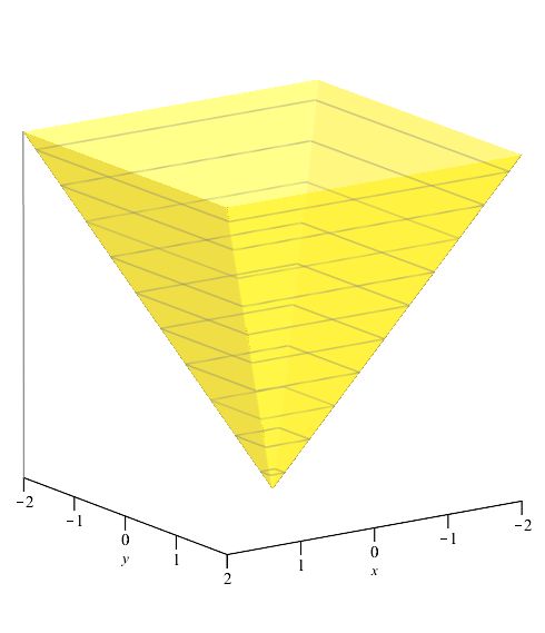
9RS2 RS1 x
S3 S2
x = RS3 RS2 RS1 x RS1 x
S1
Figure 2: The algorithm xn := ( 21 RC RB RA + 12 Id)n x0 may cycle.
remains unclear, but the explicit explanation of the connection that we have followed
is that of Daniel Gabay in 1983 [94]. In fact, clearly explaining the connection appears
to have been one of his main intentions in writing his 1983 book chapter.
Reasonable brevity precludes an in-depth discussion of Lagrangian duality beyond
establishing the connection of ADMM with Douglas–Rachford. Instead, we refer the
interested reader to a recent survey of Moursi and Yuriy Zinchenko [122], who drew
Gabay’s work to the attention of the present authors. We refer the reader also to the
sources mentioned in Remark 1.7, to Glowinski, Osher, and Yin’s recent book on split-
ting methods [101, Chapter 2], and to the following selected resources, which are by
no means comprehensive: [45, 105, 80, 106, 99, 89, 83].
1.5 Extensions to N sets
The method of alternating projections, and the associated convergence results, readily
extend to the feasibility problem for N sets
Find x ∈ ∩Nk=1 Sk , (18)
to yield the method of cyclic projections that involves iterating TS1 S2 ···SN = PSN PSN−1 · · · PS1 .
However, even for three sets the matching extension of DR,
1
xn+1 = I + RS3 RS2 RS1 (xn )
2
may cycle and so fail to solve the feasibility problem. See Figure 2, an example due to
Sims that has previously appeared in [136].
The most commonly used extension of DR from 2 sets to N sets is Pierra’s product
space method [127]. More recently Borwein and Tam have introduced a cyclic variant
[53].
101.5.1 Pierra’s Product Space Reformulation: “Divide and Concur” Method
To apply DR for finding x ∈ ∩Nk=1 Sk 6= 0,
/ we may work in the Hilbert product space
H = H N as follows.
Let S := S1 × · · · × SN
and D := {(x1 , . . . , xN ) ∈ H : x1 = x2 = · · · = xN } (19)
and apply the DR method to the two sets S and D. The product space projections for
x = (x1 , . . . , xN ) ∈ H are
PS (x1 , . . . , xN ) = (PS1 (x1 ), . . . , PSN (xN )),
!
1 N 1 N
and PD (x1 , . . . , xN ) = ∑ xk , . . . , N ∑ xk .
N k=1 k=1
The method was first nicknamed divide and concur by Simon Gravel and Veit Elser
[103]—the latter of whom credits the former for the name [81]—and the diagonal set
D in this context is referred to as the agreement set. It is clear that any point x ∈ S ∩ D
has the property that x1 = x2 = · · · = xN ∈ ∩Nk=1 Sk . It is also clear that D is a closed
subspace of H (so, PD is weakly continuous) and that, when S1 , . . . , SN are convex, so
too is S.
The form of PD and its consequent linearity allows us to readily unpack the product
space formulation to yield the iteration,
N
(xk (n + 1))Nk=1 = xk (n) − a(n) + 2A(n) − PSk (xk (n)) k=1 ,
where a(n) = N1 ∑Nk=1 xk (n) and A(n) = N1 ∑Nk=1 PSk (xk (n)), under which in the convex
case the sequence of successive iterates weakly converges (by theorem 1.5) to a limit
(x1 (∞), x2 (∞), · · · , xN (∞)) for which PSk (xk (∞)) is, for any k = 1, 2, · · · , N, a solution
to the N-set feasibility problem.
A product space schema can also be applied with AP instead of DR, to yield the
method of averaged projections,
1 N
xn+1 = ∑ Pi (xi ).
N i=1
1.5.2 Cyclic Variant: Borwein-Tam Method
The cyclic version of DR, also called the Borwein-Tam method, is defined by
T[S1 S2 ...SN ] := TSN ,S1 TSN−1 SN . . . TS2 ,S3 TS1 ,S2 , (20)
where each TSi ,S j is as defined in (3). The key convergence result is as follows.
Theorem 1.8 (Borwein & Tam, 2014). Let S1 , . . . , SN ⊂ H be closed and convex with
nonempty intersection. Let x0 ∈ H and set
xn+1 := T[S1 S2 ...SN ] xn . (21)
Then xn converges weakly to x which satisfies PS1 x = PS2 x = · · · = PSN x ∈ ∩Nk=1 Sk .
11For a proof, see [53, Theorem 3.1] or [136, Theorem 2.4.5], the latter of which—
Matthew Tam’s dissertation—is the definitive treatise on the cyclic variant.
1.5.3 Cyclically Anchored Variant (CADRA)
Bauschke, Noll, and Phan provided linear convergence results for the Borwein-Tam
method in the finite dimensional case in the presence of transversality [40]. At the same
time, they introduced the Cyclically Anchored Douglas–Rachford Algorithm (CADRA)
defined closed, convex sets A (the anchor set) and (Bi )i∈{1,...,m} where
\
A∩ Bi 6= 0/
i∈{1,...,m}
\
and (∀i ∈ {1, . . . , m})Ti = PBi RA + Id − PA , Zi = Fix Ti , Z= Zi .
i∈{1,...,m}
where (∀n ∈ N) xn+1 := T xn where T := Tm . . . T2 T1 . (22)
When m = 1, CADRA becomes regular DR, which is not the case for the Borwein-Tam
method. The convergence result is as follows.
Theorem 1.9. CADRA (Bauschke, Noll, Phan, 2015 [40, Theorem 8.5]) The sequence
(xn )n∈N from (22) converges weakly to x ∈ Z with PA x ∈ A ∩ i∈{1,...,m} Bi . Convergence
T
is linear if one of the following hold:
1. X is finite-dimensional and riA ∩ 6= 0/
T
i∈{1,...,m} riBi
2. A and each Bi is a subspace with A+Bi closed and that (Zi )i∈{1,...,m} is boundedly
linearly regular.
1.5.4 String-averaging and block iterative variants
In 2016, Yair Censor and Rafiq Mansour introduced the string-averaging DR (SA-DR)
and block-iterative DR (BI-DR) variants [61]. SA-DR involves separating the index
set I := {1, . . . , N} (where N is as in (18)) into strings along which the two-set DR
operator is applied and taking a convex combination of the strings’ endpoints to be the
next iterate. Formally, letting It := (it1 , it2 , . . . , itγ(t) ) be an ordered, nonempty subset of I
with length γ(t) for t = 1, . . . , M and x0 ∈ H, set
M M
xk+1 := ∑ wt Vt (xk ) with wt > 0 (∀t = 1, . . . , M) and ∑ wt = 1
t=1 t=1
where Vt (xk ) :=Tit ,it Tit −1,itγ(t) . . . Tit2 ,it3 Tit1 ,it2 (xk ),
γ(t) 1 γ(t)
where TA,B is the 2-set DR operator. The principal result is as follows.
Theorem 1.10. SA-DR (Censor & Mansour, 2016 [61, Theorem 18]) Let S1 , . . . , SN ⊂
H be closed and convex with int ∩i∈I Si 6= 0.
/ Then for any x0 ∈ H, any sequence (xk )∞
k=1
generated by the SA-DR algorithm with strings satisfying I = I1 ∪I2 ∪· · ·∪IM converges
strongly to a point x∗ ∈ ∩i∈I Si .
12The BI-DR algorithm involves separating I into subsets and applying 2-set DR to
each of them by choosing a block index according to the rule tk = k mod M + 1 and
setting
γ(tk ) γ(tk )
t t
xk+1 := ∑ w jk z j with wtk > 0 (∀ j = 1, . . . , γ(tk )) and ∑ w jk = 1,
j=1 j=1
where z j :=Titk ,itk (xk ) (∀ j = 1, . . . , γ(tk ) − 1) and zγ(tk ) := Titk t
,i k
(xk ).
j j+1 γ(tk ) 1
The principal result is as follows.
Theorem 1.11. BI-DR (Censor & Mansour, 2016 [61, Theorem 19]) Let S1 , . . . , SN ⊂
H be closed and convex with ∩i∈I Si 6= 0.
/ For any x0 ∈ H, the sequence (xk )∞ k=1 of iter-
ates generated by the BI-DR algorithm with I = I1 ∪ · · · ∪ IM , after full sweeps through
all blocks, converges
1. weakly to a point x∗ such that PSit (x∗ ) ∈ ∩ j=1 Sitj for j = 1, . . . , γ(t) and t =
γ(t)
j
1, . . . , M, and
2. strongly to a point x∗ such that x∗ ∈ ∩Ni=1 Si if the additional assumption int ∩i∈I
Si 6= 0/ holds.
1.5.5 Cyclic r-sets DR: Aragón Artacho-Censor-Gibali Method
Motivated by the intuition of the Borwein-Tam method and the example in Figure 2,
Francisco Aragón Artacho, Censor, and Aviv Gibali have recently introduced another
method which simplifies to classical Douglas–Rachford method in the 2-set case [12,
Theorem 3.7].
For the feasibility problem of N sets S0 , . . . , SN−1 , we denote by SN,r (d) the finite
sequence of sets:
SN,r (d) := S((r−1)d−(r−1))mod N , S((r−1)d−(r−2))mod N , . . . , S((r−1)d)mod N .
The method is then given by
xn+1 := VN VN−1 . . . V1 (xn ).
1
where Vd := Id +VCm,r (d)
2
and VC0 ,C1 ,...,Cr−1 := RCr−1 RCr−2 RC0 .
Provided the condition int ∩N−1
i=0 Si 6= 0,
/ the sequence (xn )∞
n=1 converges weakly to
a solution of the feasibility problem. They also provided a more general result, [12,
Theorem 3.4], whose sufficiency criteria are, generically, more difficult to verify.
131.5.6 Sums of N Operators: Spingarn’s Method
One popular method for finding a point in the zero set of a sum of N monotone opera-
tors T1 , . . . , TN is the reduction to a 2 operator problem given by
A :=T1 ⊗ T2 ⊗ · · · ⊗ TN (23)
B :=NB (24)
where NB is the normal cone operator (8) for B and B is the agreement set defined
in (19). As A and B are maximal monotone, the weak convergence result is given
by Svaiter’s relaxation [134] of Theorem 1.4. The application of DR to this problem
is analogous to the product space method discussed in 1.5.1. In 2007 Eckstein and
Svaiter [79] described this as Spingarn’s method, referencing Spingarn’s 1983 article
[132]. They also established a general projective framework for such problems which
does not require reducing the problem to the case N = 2.
2 Convex Setting
Throughout the rest of the exposition, we will take the Douglas–Rachford operator and
sequence to be as in (5). Where no mention is made of the parameters λ , µ, γ, it is un-
derstood that they are as in Definition 1.2. While Theorems 1.5 and 1.4 guarantee weak
convergence for DR in the convex setting, only in finite dimensions is this sufficient to
guarantee strong convergence. An important result of Hundal shows that AP may not
converge in norm for the convex case when H is infinite dimensional [110] (see also
[20, 119]). Although no analogue of Hundal’s example seems known, to date, for DR
in the infinite dimensional case norm convergence has been verified under additional
assumptions on the nature of A and B.
2.1 Convergence
Borwein, Li, and Tam [48] attribute the first convergence rate results for DR to Hesse,
Luke, and Patrick Neumann who in 2014 showed local linear convergence in the pos-
sibly nonconvex context of sparse affine feasibility problems [109]. Bauschke, Bello
Cruz, Nghia, Phan, and Wang extended this work by showing that the rate of linear
convergence of DR for subspaces is the cosine of the Friedrichs angle [17].
In 2014, Bauschke, Bello Cruz, Nghia, Phan, and Wang [25] used the convergence
rates of matrices to find optimal convergence rates of DR for subspaces with more gen-
eral averaging parameters as in (5). In 2017, Mattias Fält and Giselsson characterized
the parameters that optimize the convergence rate in this setting [87].
In 2014, Pontus Giselsson and Stephen Boyd demonstrated methods for precondi-
tioning a particular class of problems with linear convergence rate in order to optimize
a bound on the rate [97].
Motivated by the recent local linear convergence results in the possibly nonconvex
setting [108, 109, 126, 115], Borwein, Li, and Tam asked whether a global convergence
rate for DR in finite dimensions might be found for a reasonable class of convex sets
14even when the regularity condition riA ∩ riB 6= 0/ is potentially not satisfied. They pro-
vided some partial answers in the context of Hölder regularity with special attention
given to convex semi-algebraic sets [48].
Borwein, Sims, and Tam established sufficient conditions to guarantee norm con-
vergence in the setting where one set is the positive Hilbert cone and the other set a
closed affine subspace which has finite codimension [51].
In 2015, Bauschke, Dao, Noll, and Phan studied the setting of R2 where one set is
the epigraph of a convex function and the other is the real axis, obtaining various con-
vergence rate results [31]. In their follow-up article in 2016, they demonstrated finite
convergence when Slater’s condition holds in both the case where one set is an affine
subspace and the other a polyhedron and in the case where one set is a hyperplane and
the other an epigraph [30]. They included an analysis of the relevance of their results
in the product space setting of Spingarn [132] and numerical experiments comparing
the performance of DR and other methods for solving linear equations with a positivity
constraint. In the same year, Bauschke, Dao, and Moursi provided a characterization
of the behaviour of the sequence (T n x − T n y)n∈N [28].
In 2015, Damek Davis and Wotao Yin showed that DR might converge arbitrarily
slowly in the infinite dimensional setting [70].
2.1.1 Order of operators
In 2016, Bauschke and Moursi investigated the order of operators: TA,B vs. TB,A . In so
doing, they demonstrated that RA : Fix TA,B → Fix TB,A and RB : Fix TB,A → Fix TA,B are
bijections [37].
2.1.2 Best approximations and the possibly infeasible case
The behaviour of DR in the inconsistent setting is most often studied using the minimal
displacement vector
v := Pran(Id−TA,B ) 0. (25)
The set of best approximation solutions relative to A is A∩(v+B); when it is nonempty,
the following have also been shown.
In 2004 Bauschke, Combettes, and Luke considered the algorithm under the name
averaged alternating reflections (AAR). They demonstrated that in the possibly incon-
sistent case, the shadow sequence PA xn remains bounded with its weak sequential clus-
ter points being in A ∩ (v + B) [24].
In 2015, Bauschke and Moursi [36] analysed the more specific setting of two affine
subspaces, showing that PA xn will converge to a best approximation solution. In 2016,
Bauschke, Minh Dao, and Moursi [29] furthered this work by considering the affine-
convex setting, showing that when one of A and B is a closed affine subspace PA xn will
converge to a best approximation solution. They then applied their results to solving
the least squares problem of minimizing ∑M 2
k=1 dCk (x) with Spingarn’s splitting method
[132].
In 2016, Bauschke and Moursi provided a more general sufficient condition for
the weak convergence [38], and in 2017 they characterized the magnitudes of mini-
15mal displacement vectors for more general compositions and convex combinations of
operators.
2.1.3 Nearest feasible points (Aragón Artacho-Campoy Method)
In 2017, Aragón Artacho and Campoy introduced what they called the Averaged Al-
ternating Modified Reflections (AAMR) method for finding the nearest feasible point
for a given starting point [10]. The operator and method are defined with parameters
α, β ∈]0, 1[ by
TA,B,α,β := (1 − α)Id + α(2β PB − Id)(2β PA − Id)
xn := TA−q,B−q,α,β xn , n = 0, 1, . . . (26)
which we recognize as DR in the case α = 1/2, β = 1, q = 0. The convergence result
is as follows.
Theorem 2.1. Aragón Artacho & Campoy 2017, [10, Theorem 4.1] Given A, B closed
and convex, α, β ∈]0, 1[, and q ∈ H, choose any x0 ∈ H. Let (xn )n∈N be as in (26).
Then if A ∩ B 6= 0/ and q − PA∩B (q) ∈ (NA + NB )(PA∩B (q)) then the following hold:
1. (xn )n∈N is weakly convergent to a point x ∈ Fix TA−q,B−q,α,β such that PA (q+x) =
PA∩B (q);
2. (xn+1 − xn )n∈N is strongly convergent to 0;
3. (PA (q + xn ))n∈N is strongly convergent to PA∩B (q).
Otherwise kxn k → ∞. Moreover, if A, B are closed affine subspaces, A ∩ B 6= 0,
/ and q −
PA∩B (q) ∈ (A−A)⊥ +(B−B)⊥ then (xn )n∈N is strongly convergent to PFix TA−q,B−q,α,β (x0 ).
The algorithm may be thought of as another approach to the convex optimization
problem of minimizing the convex function y 7→ kq − yk2 subject to constraints on the
solution.
It is quite natural to consider the theory of the algorithm in the case where projec-
tion operators PA = JNA , PB = JNB are replaced with more general resolvents for maxi-
mally monotone operators [9], an extension Aragón Artacho and Campoy gave in 2018.
This work has already been extended by Alwadani, Bauschke, Moursi, and Wang, who
analysed the asymptotic behaviour and gave the algorithm the more specific name of
Aragón Artacho-Campoy Algorithm (AACA) [2].
2.1.4 Cutter methods
Another computational approach is to replace true projections with approximate pro-
jections or cutter projections onto separating hyperplanes as in Figure 3a. Prototyp-
ical of this category are subgradient projection methods which may be used to find
x ∈ ∩mi=1 lev≤0 f i for m convex functions f 1 , . . . , f m ; see Figure 3b. Such methods are
not generally nonexpansive (as shown in 3b) but may be easier to compute. When true
reflection parameters are allowed, the method is no longer immune from “bad” fixed
16HB HA
RB RA x
x
TA,B x
PA x PB RA x B
RA x A x0
Pf x1 Pf x2x1 x2
(a) DR with cutters (b) Subgradient projectors (c) A fixed point of subgra-
may not be nonexpansive dient DR
Figure 3: Cutter methods
points, as illustrated in Figure 3c. However, with a suitable restriction on reflection pa-
rameters and under other modest assumptions, convergence may be guaranteed through
Fejér monotonicity methods. See, for example, the works of Cegielski and Fukushima
[60, 92]. More recently, Díaz Millán, Lindstrom, and Roshchina have provided a stan-
dalone analysis of DR with cutter projections [73].
2.2 Notable Applications
While the Douglas–Rachford operator is firmly nonexpansive in the convex setting, the
volume of literature about it is expansive indeed. While reasonable brevity precludes
us from furnishing an exhaustive catalogue, we provide a sampling of the relevant
literature.
As early as 1961, working in the original context of Douglas and Rachford, P.L.T.
Brian introduced a modified version of DR for high order accuracy solutions of heat
flow problems [58].
In 1995, Fukushima applied DR to the traffic equilibrium problem, comparing
its performance (and the complexity and applicability of the induced algorithms) to
ADMM [93].
In 2007, Combettes and Jean-Christophe Pesquet applied a DR splitting to nons-
mooth convex variational signal recovery, demonstrating their approach on image de-
noising problems [64].
In 2009, Simon Setzer showed that the Alternating Split Bregman Algorithm from
[102] could be interpreted as a special case of DR in order to interpret its convergence
properties, applying the former to an image denoising problem [131]. In the same
year, Gabriele Steidl and Tanja Teuber applied DR for removing multiplicative noise,
analysing its linear convergence in their context and providing computational examples
by denoising images and signals [133].
In 2011 Combettes and Jean-Christophe Pesquet contrasted and compared various
proximal point algorithms for signal processing [65].
In 2012 Laurent Demanet and Xiangxiong Zhang applied DR to l1 minimization
problems with linear constraints, analysing its convergence and bounding the conver-
17gence rate in the context of compressed sensing [72].
In 2012, Radu Ioan Boţ, and Christopher Hendrich proposed two algorithms based
on Douglas–Rachford splitting, which they used to solve a generalized Heron problem
and to deblur images [55]. In 2014, they analysed with Ernö Robert Csetnek an inertial
DR algorithm and used it to solve clustering problems [54].
In 2015, Bauschke, Valentin Koch, and Phan applied DR for a road design opti-
mization problem in the context of minimizing a sum of proper convex lsc functions,
demonstrating its effectiveness on real world data [34].
In 2017, Fei Wang, Greg Reid, and Henry Wolkowicz applied DR with facial re-
duction for a set of matrices of a given rank and a linear constraint set in order to find
maximum rank moment matrices [139].
3 Non-convex Setting
Investigation in the nonconvex setting has been two-pronged, with the theoretical in-
quiry chasing the experimental discovery. The investigation has also taken place in,
broadly, two contexts: that of curves and/or hypersurfaces and that of discrete sets.
While Jonathan Borwein’s exploration spanned both of the aforementioned con-
texts, his interest in DR appears to have been initially sparked by its surprising perfor-
mance in the latter [81], specifically the application of the method by Elser, Ranken-
burg, and Thibault to solving a wide variety of combinatorial optimization problems,
including Sudoku puzzles [86]. Where the product space reformulation is applied to
feasibility problems with discrete constraint sets, DR often succeeds while AP does
not. Early wisdom suggested that one reason for its superior performance is that DR,
unlike AP, is immune from false fixed points regardless of the presence or absence of
convexity, as shown in the following proposition (see, for example, [136, Proposition
1.5.1] or [86]).
Proposition 3.1 (Fixed points of DR). Let A, B ⊂ H be proximal. Then x ∈ Fix TA,B
implies PA (x) ∈ A ∩ B.
Proof. Let x ∈ Fix TA,B . Then x = x + PB (2PA (x) − x) − PA (x) and so PB (2PA (x) − x) −
PA (x) = 0, so PA (x) ∈ B.
A typical example where A := {a1 , a2 } is a doubleton and B a subspace (analogous
to the agreement set) is illustrated in Figure 4 where DR is seen to solve the problem
while AP becomes trapped by a fixed point.
If the germinal work on DR in the nonconvex setting is that of Elser, Rankenburg,
and Thibault [86] (caution: the role of A and B are reversed from those here), then
the seminal work is that of J.R. Fienup who applied the method to solve the phase re-
trieval problem [88]. In [86], Elser et al. referred to DR as Fienup’s iterated map and
the difference map, while Fienup himself called it the hybrid input-output algorithm
(HIO) [88]. Elser explains that, originally, neither Fienup nor Elser et al. were aware
of the work of Lions and Mercier [117], and so the seminal work on DR in the non-
convex setting is, surprisingly, an independent discovery of the method [81]. Fienup
18x0 x0
B B
x7
x1 a1 xn for n ≥ 1
a1
a2 a2
xn for n ≥ 8 PA xn for n ≥ 8 R
(a) DR (b) AP
Figure 4: DR and AP for a doubleton and a line in R2
constructed the method by combining aspects of two other methods he considered—
the basic input-output algorithm and the output-output algorithm—with the intention
of obviating stagnation. Here again, one may think of the behaviour illustrated in Fig-
ure 4.
(a) Convergence to a feasible (b) Convergence to a fixed point (c) Proof of convergence with
point Benoist’s Lyapunov function
Figure 5: Behaviour of DR where A is a circle and B is a line; (c) is discussed in 3.2.
Figure 5 shows behaviour of DR in the case where A is a circle and B is a line,
a situation prototypical of the phase retrieval problem. For most arrangements, DR
converges to a feasible point as in Figure 5a. However, when the line and circle meet
tangentially as in Figure 5b, DR converges to a fixed point which is not feasible, and
the sequence PA xn converges to the true solution.
Elser notes that it is unclear whether or not Fienup understood that a fixed point of
the algorithm is not necessarily feasible, as his approach was largely empirical. Elser
sought to clarify this point in his follow up article in which he augmented the study
19of DR for phase retrieval by replacing support constraints with object histogram and
atomicity constraints for crystallographic phase retrieval [82, Section 5]. In 2001 when
[82] was submitted, Elser was not yet aware of Lions’ and Mercier’s characterization
of DR as the Douglas–Rachford method; it may be recognized in [82] as a special
instance of the difference map (which we define in (27)), a generalization of Fienup’s
input-output map.
In 2002, Bauschke, Combettes, and Luke finally demonstrated that Fienup’s ba-
sic input-output algorithm is an instance of Dykstra’s algorithm and that HIO (Hybrid
Input–Output) with the support constraint alone corresponds to DR [22] (see also their
2003 follow up [23]). In another follow up [24], they showed that with support and
nonnegativity constraints, HIO corresponds to the HPR (hybrid projection reflection)
algorithm, a point Luke sought to clarify in his succinct 2017 summary of the investi-
gation of DR in the context of phase retrieval [118].
More recently, in 2017, Elser, Lan, and Bendory have published a set of bench-
mark problems for phase retrieval [85]. They considered DR with true reflections
and a relaxed averaging parameter—µ = γ = 0, λ ∈]0, 1] as in (5)—under the name
relaxed-reflect-reflect (RRR). In particular, they provided experimental evidence for the
exponential growth of DR’s mean iteration count as a function of the autocorrelation
sparsity parameter, which seems well-suited for revealing behavioural trends. They
also provided an important clarification of the different algorithms which have been
labelled “Fienup” algorithms in the literature, some of which are not DR.
3.1 Discrete Sets
The landmark experimental work on discrete sets is that of Elser, Rankenburg, and
Thibault [86]. They considered the performance of what they called the difference map
for various values of the parameter β :
T : x 7→ x + β (PA ◦ fB (x) − PB ◦ fA (x)) , (27)
where fA : x 7→ PA (x) − (PA (x) − x) /β ,
and fB : x 7→ PB (x) + (PB (x) − x) /β .
When β = −1, we recover the DR operator TA,B , and when β = 1, we obtain TB,A .
3.1.1 Stochastic Problems
Much of the surprising success of DR has been in the setting where some of the sets of
interest have had the form {0, 1} p . Elser et al. adopted the approach of using stochastic
feasibility problems to study the performance of DR [86]. They began with the problem
of solving the linear Diophantine equation Cx = b, where C, a stochastic p × q matrix,
and b ∈ N p are “known.” Requiring the solution x ∈ {0, 1}q that is used to generate
the problem to also be stochastic ensures uniqueness of the solution for the feasibility
problem: find x ∈ A ∩ B where
A := {0, 1}q , and B := {x ∈ Rq such that Cx = b}.
20They continued by solving Latin squares of n symbols. Where xi jk = 1 indicates that
the cell in the ith row of the jth column of the square is k, the problem is stochastic and
the constraint that xî jˆk̂ = 1 if and only if (∀i 6= î) xi jˆk̂ = 0, (∀ j 6= jˆ)xî jk̂ = 0 determines
the set of allowable solutions. The most familiar form of a Latin square is the Sudoku
puzzle where n = 9 and we require the additional constraint that the complete square
consist of a grid of 9 smaller Latin squares. For more on the history of the application
of projection algorithms to solving Sudoku puzzles, see Schaad’s master’s thesis [130]
in which he also applies the method to the 8 queens problem .
This work of Elser et al. piqued the interest of Jonathan Borwein who in 2013, to-
gether with Aragón Artacho and Matthew Tam, continued the investigation of Sudoku
puzzles [6, 4], exploring the effect of formulation (integer feasibility vs. stochastic) on
performance. They also extended the approach by solving nonogram problems.
3.1.2 Matrix completion and decomposition
Another application for which DR has shown promising results is finding the remain-
ing entries of a partially specified matrix in order to obtain a matrix of a given type.
Borwein, Aragón Artacho, and Tam considered the behaviour of DR for such matrix
completion problems [5]. They provided a discussion of the convex setting, including
positive semidefinite matrices, correlation matrices, and doubly stochastic matrices.
They went on to provide experimental results for a number of nonconvex problems,
including for rank minimization, protein reconstruction, and finding Hadamard and
skew-Hadamard matrices. In 2017, Artacho, Campoy, Kotsireas, and Tam applied
DR to construct various classes of circulant combinatorial designs [11], reformulating
them as three set feasibility problems. Designs they studied included Hadamard ma-
trices with two circulant cores, as well as circulant weighing matrices and D-optimal
matrices.
Even more recently, David Franklin used DR to find compactly supported, non-
separable wavelets with orthonormal shifts, subject to the additional constraint of regu-
larity [91, 90]. Reformulating the search as a three set feasibility problem in {C2×2 }M
for M = {4, 6, 8, . . . }, they compared the performance of cyclic DR, product space DR,
cyclic projections, and the proximal alternating linear minimisation (or PALM) algo-
rithm. Impressively, product space DR solved every problem it was presented with.
In 2017, Elser applied DR—under the name RRR (short for relaxed reflect-reflect)—
for matrix decomposition problems, making several novel observations about DR’s ten-
dency to wander, searching in an apparently chaotic manner, until it happens upon the
basin for a fixed point [83]. These observations have motivated the open question we
pose in 4.1.2.
3.1.3 The study of proteins
In 2014, Borwein and Tam went on to consider protein conformation determination, re-
formulating such problems as matrix completion problems [52]. An excellent resource
for understanding the early class problems studied by Borwein, Tam, and Aragón
Artacho—as well as the cyclic DR algorithm described in subsection 1.5—is Tam’s
PhD dissertation [136].
21Elser et al. applied DR to study protein folding problems, discovering much faster
performance than that of the landscape sampling methods commonly used [86].
3.1.4 Where A is a subspace and B a restriction of allowable solutions
Elser et al. applied DR to the study of 3-SAT problems, comparing its performance to
that of another solver, Walksat [86] (see also [103]). They found that DR solved all
instances without requiring random restarts. They also applied the method to the spin
glass ground state problem, an integer quadratic optimization program with nonpositive
objective function.
3.1.5 Graph Coloring
Elser et al. applied DR to find colorings of the edges of complete graphs with the con-
straint that no triangle may have all its edges of the same color [86]. They compared its
performance to CPLEX, and included an illustration showing the change of edge colors
over time. DR solved all instances, and outperformed CPLEX in harder instances.
In 2016, Francisco Aragón Artacho and Rubén Campoy applied DR to solving
graph coloring problems in the usual context of coloring nodes [8]. They constructed
the feasibility problem by attaching one of two kinds of gadgets to the graphs, and they
compared performance with the two different gadget types both with and without the
inclusion of maximal clique information. They also explored the performance for sev-
eral other problems reformulated as graph coloring problems; these included: 3-SAT,
Sudoku puzzles, the eight queens problem and generalizations thereof, and Hamilto-
nian path problems.
More recently, Aragón Artacho, Campoy, and Elser [14] have considered a refor-
mulation of the graph coloring problem based on semidefinite programming, demon-
strating its superiority through numerical experimentation.
3.1.6 Other implementations
Elser et al. went on to consider the case of bit retrieval, where A is a Fourier magni-
tude/autocorrelation constraint and B is the binary constraint set {±1/2}n [86]. They
found its performance to be superior to that of CPLEX.
Bansal used DR to solve Tetravex problems [16].
More recently, in 2018, Elser expounded further upon the performance of DR under
varying degrees of complexity by studying its behaviour on bit retrieval problems [84].
Of his findings of its performance he observes:
These statistics are consistent with an algorithm that blindly and repeat-
edly reaches into an urn of M solution candidates, terminating when it has
retrieved one of the 4 × 43 solutions. Two questions immediately come to
mind. The easier of these is: How can an algorithm that is deterministic
over most of its run-time behave randomly? The much harder question is:
How did the M = 243 solution candidates get reduced, apparently, to only
about 1.7 × 105 × (4 × 43) ≈ 224 ?
22The behaviour of DR under varying complexity remains a fascinating open topic,
and we provide it as one of our two open problems in 4.1.2.
3.1.7 Theoretical Analysis
One of the first global convergence results in the nonconvex setting was given by
Aragón Artacho, Borwein, and Tam in the setting where one set is a half space and
the second set finite [7]. Bauschke, Dao, and Lindstrom have since fully categorized
the global behaviour for the case of a hyperplane and a doubleton (set of two points)
[27]. Both problems are prototypical of discrete combinatorial feasibility problems,
the latter especially insofar as the hyperplane is analogous to the agreement set in the
product space version of the method discussed in section 1.5.1, the most commonly
employed method for problems of more than 2 sets.
3.2 Hypersurfaces
In 2011, Borwein and Sims made the first attempt at deconstructing the behaviour of
DR in the nonconvex setting of hypersurfaces [50]. In particular, they considered in
detail the case of a circle A and a line B, a problem prototypical of phase retrieval.
Here the dynamical geometry software Cinderella [1] first played an important role in
the analysis: the authors paired Cinderella’s graphical interface with accurate compu-
tational output from Maple in order to visualize the behaviour of the dynamical system.
Borwein and Sims went on to show local convergence in the feasible case where the
line is not tangent to the 2-sphere by using a theorem of Perron. They concluded by
suggesting analysis for a generalization of the 2-sphere: p-spheres.
In 2013 Aragón Artacho and Borwein revisited the case of a 2-sphere and line
intersecting non-tangentially [3]. When x0 lies in the subspace perpendicular to B, the
sequence (xn )∞n=0 is contained in the subspace and exhibits chaotic behaviour. For x0
not in the aforementioned subspace—which we call the singular set—they provided
a conditional proof of global convergence of iterates to the nearer of the two feasible
points. The proof relied upon constructing and analysing the movement of iterates
through different regions. Borwein humorously remarked of the result that, “This was
definitely not a proof from the book. It was a proof from the anti-book.” Joël Benoist
later provided an elegant proof of global convergence by constructing the Lyapunov
function seen in Figure 5c [44].
In one of his later posthumous publications on the subject [46], Borwein, together
with Ohad Giladi, demonstrated that the DR operator for a sphere and a convex set may
be approximated by another operator satisfying a weak ergodic theorem.
In 2016, Borwein, Lindstrom, Sims, Skerrit, and Schneider undertook Borwein’s
suggested follow up work in R2 , analysing not only the case of p-spheres more gener-
ally but also of ellipses [49]. They discovered incredible sensitivity of the global be-
haviour to small perturbations of the sets, with some arrangements eliciting a complex
and beautiful geometry characterized by periodic points with corresponding basins of
attraction. A point x satisfying T n x = x is said to be periodic with period the smallest
n for which this holds; Figure 6 from [49] shows 13 different DR sequences for an
ellipse and line from which subsequences converge to periodic points. Borwein et al.
23You can also read