Theory of Proton-Proton Collisions - James Stirling IPPP, Durham University
←
→
Page content transcription
If your browser does not render page correctly, please read the page content below
Theory of Proton-Proton
      Collisions

      James Stirling
  IPPP, Durham University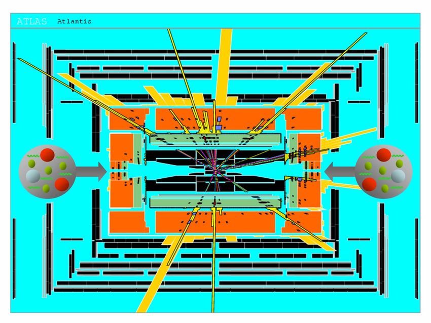
references
“QCD and Collider Physics”

RK Ellis, WJ Stirling, BR Webber
Cambridge University Press (1996)

also

“Handbook of Perturbative QCD”

G Sterman et al (CTEQ Collaboration)
www.phys.psu.edu/~cteq/

                           SSI 2006    2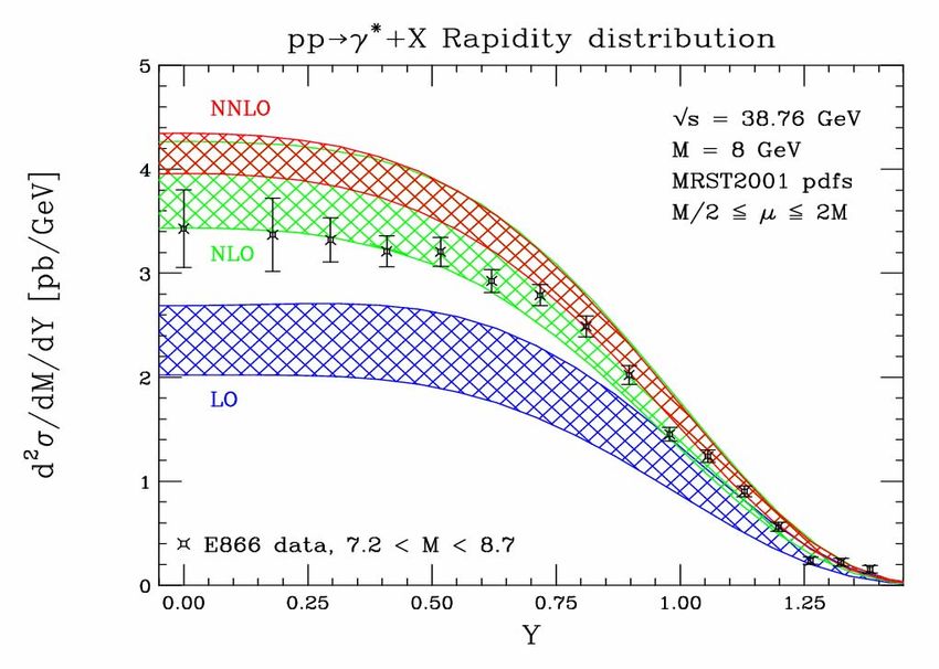
… and
“Hard Interactions of
Quarks and Gluons: a
Primer for LHC Physics ”

JM Campbell, JW Huston, WJ
Stirling (CSH)

www.pa.msu.edu/~huston/semi
nars/Main.pdf

to appear in Rep. Prog. Phys.

                            SSI 2006   3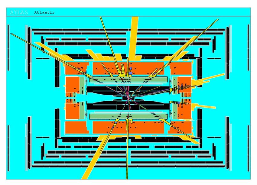
past, present and future proton/antiproton
                  colliders…
             Tevatron (1987→)
                       Fermilab
   proton-antiproton collisions
             √S = 1.8, 1.96 TeV

  -
SppS (1981 → 1990)
CERN
proton-antiproton
collisions                               LHC (2007 → )
√S = 540, 630 GeV                        CERN
                                         proton-proton and
                                         heavy ion collisions
                                         √S = 14 TeV

                              SSI 2006                   4
discoveries
       c b W,Z          t             H, SUSY?

1970     1980    1990       2000        2010     2020

                    Higgs discovery
                        at LHC

                    SUSY discovery
                       at LHC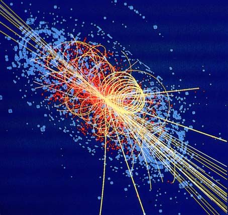
What can we calculate?

Scattering processes at high energy
hadron colliders can be classified as
either HARD or SOFT

Quantum Chromodynamics (QCD) is
the underlying theory for all such
processes, but the approach (and the
level of understanding) is very different
for the two cases

For HARD processes, e.g. W or high-
ET jet production, the rates and event
properties can be predicted with some
precision using perturbation theory

For SOFT processes, e.g. the total
cross section or diffractive processes,
the rates and properties are dominated
by non-perturbative QCD effects, which
are much less well understood
                                      SSI 2006   6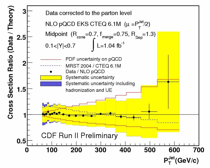
Outline
•   Basics: QCD, partons, pdfs
     – basic parton model ideas for DIS
     – scaling violation & DGLAP
     – parton distribution functions
•   Application to hadron colliders
     – hard scattering & basic kinematics
     – the Drell Yan process in the parton model
     – order αS corrections to DY, singularities, factorisation
     – examples of other hard processes and their phenomenology
     – parton luminosity functions
     – uncertainties in the calculations
•   Beyond fixed-order inclusive cross sections
     – Sudakov logs and resummation
     – parton showering models (basic concepts only!)
     – the role of non-perturbative contributions: intrinsic kT,
     – underlying event/minimum bias contributions
     – theoretical frontiers: exclusive production of Higgs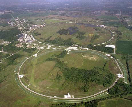
Basics of QCD

gluon             gluon                 αS(μ)   non-perturbative
        gS Taij             gS fabc
                                           1

quark     quark   gluon     gluon                        perturbative
                          αS = gS2/4π       0
                                                           μ (GeV)
• renormalisation of the coupling

• colour matrix algebra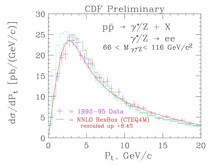
Asymptotic Freedom

           “What this year's Laureates
           discovered was something that, at
           first sight, seemed completely
           contradictory. The interpretation of
           their mathematical result was that the
           closer the quarks are to each other,
           the weaker is the 'colour charge'.
           When the quarks are really close to
           each other, the force is so weak that
           they behave almost as free particles.
           This phenomenon is called
           ‘asymptotic freedom’. The converse
           is true when the quarks move apart:
           the force becomes stronger when the
           distance increases.”

                 αS(r)

SSI 2006                       1/r           9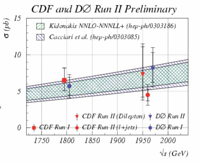
deep inelastic scattering and the
            parton model
electron                             • variables
                 qμ                  Q2 = –q2 (resolution)
                         pμ
           X                         x = Q2 /2p·q (inelasticity)
                         proton
                                                   1.2
                                                                                                2     2
                                                                                            Q (GeV )

• structure functions                              1.0
                                                                                                1.5
                                                                                                3.0
                                                                                                5.0
                                                   0.8                                          8.0

dσ/dxdQ2 ∝     α2 Q-4   (x,Q2)
                                                                                                11.0
                  F2                    F2(x,Q )
                                        2
                                                   0.6
                                                                                                8.75
                                                                                                24.5

• (Bjorken) scaling                                0.4
                                                                                                230
                                                                                                80
                                                                                                800
                                                                                                8000

F2(x,Q2) → F2(x) (SLAC, ~1970)                     0.2

                                                   0.0
                                                      0.0   0.1   0.2   0.3   0.4   0.5   0.6       0.7   0.8

               Bjorken 1968       SSI 2006                                                                      10
the parton model (Feynman 1969)
• photon scatters incoherently off massless, infinite
momentum
pointlike, spin-1/2 quarks frame
• probability that a quark carries fraction ξ of parent
proton’s momentum is q(ξ), (0< ξ < 1)
∑ ∫ dξ ∑
1
F2 ( x) = eq2 ξ q(ξ ) δ ( x − ξ ) = eq2 x q ( x)
0
q ,q q ,q
4 1 1
= x u ( x) + x d ( x) + x s ( x) + ...
9 9 9
• the functions u(x), d(x), s(x), … are called parton
distribution functions (pdfs) - they encode
information about the proton’s deep structure
SSI 2006 11extracting pdfs from experiment
• different beams
(e,μ,ν,…) & targets
(H,D,Fe,…) measure 4 1 1
F2ep = (u + u ) + ( d + d ) + ( s + s) + ...
different combinations of 9 9 9
quark pdfs 1 4 1
F2en = (u + u ) + (d + d ) + ( s + s ) + ...
• thus the individual q(x)
F2νp
9
[
9
= 2 d + s + u + ... ]
9
can be extracted from a
set of structure function F2νn = 2 [u + d + s + ...]
•
measurements
gluon not measured 5 νN
s = s = F2 − 3F2eN
directly, but carries 6
about 1/2 the proton’s
momentum ∑ ∫ dx x (q( x) + q( x)) = 0.55
1
q 0
SSI 2006 1235 years of Deep Inelastic Scattering
1.2
2 2
Q (GeV )
1.0
1.5
3.0
5.0
0.8 8.0
11.0
8.75
F2(x,Q )
2
0.6 24.5
230
80
0.4
800
8000
0.2
0.0
0.0 0.1 0.2 0.3 0.4 0.5 0.6 0.7 0.8
SSI 2006 13(MRST) parton distributions in the proton
1.2
MRST2001 up
1.0 2
Q = 10 GeV
2 down
antiup
antidown
0.8
strange
charm
x f(x,Q )
2
0.6 gluon
0.4
0.2
0.0
-3 -2 -1 0
10 10 10 10
x Martin, Roberts, S, Thorne
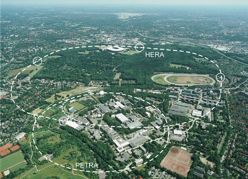
SSI 2006 14HERA e+, e− (28 GeV) p (920 GeV)
a deep inelastic scattering event at HERA

   quark

electron                             proton
35 years of Deep Inelastic Scattering
           1.2
                                                             2     2
                                                         Q (GeV )
           1.0
                                                             1.5
                                                             3.0
                                                             5.0
           0.8                                               8.0
                                                             11.0
                                                             8.75
F2(x,Q )
2

           0.6                                               24.5
                                                             230
                                                             80
           0.4
                                                             800
                                                             8000
           0.2

           0.0
              0.0   0.1   0.2   0.3       0.4    0.5   0.6       0.7   0.8

                                      SSI 2006                               17
scaling violations and QCD
The structure function data exhibit systematic violations
of Bjorken scaling:
6
4
F2 Q2 > Q1
2
Q1
quarks emit gluons!
0
0.0 0.2 0.4 0.6 0.8 1.0
x
SSI 2006 18+ + + +…
where the logarithm comes from
(‘collinear singularity’) and
then convolute with a ‘bare’ quark distribution in the proton:
q0(x)
p xpnext, factorise the collinear divergence into a ‘renormalised’
quark distribution, by introducing the factorisation scale μ2 :
then finite, by construction
note arbitrariness of ‘factorisation scheme dependence’
_
we can choose C such that Cq= 0, the DIS scheme,__ or use dimensional
regularisation and remove the poles at N=4, the MS scheme, with Cq ≠ 0
q(x,μ2) is not calculable in perturbation theory,* but its scale (μ2)
dependence is: Dokshitzer
Gribov
Lipatov
Altarelli
Parisi
*lattice QCD?note that we are free to choose μ2 = Q2 in which case
coefficient function,
see QCD book
… and thus the scaling violations of the structure function
follow those of q(x,Q2) predicted by the DGLAP equation:
6
4 Q2 > Q1
q
F2
2
Q1
0
0.0 0.2 0.4 0.6 0.8 1.0
x
the rate of change of F2 is proportional to αS
(DGLAP), hence structure function data can be
used to measure the strong coupling!however, we must also include
the gluon contribution
coefficient functions
- see QCD book
… and with additional terms in the DGLAP equations
note that at small (large) x, the splitting
functions
gluon (quark) contribution
dominates the evolution of the
quark distributions, and therefore
of F2DGLAP evolution: physical picture
Altarelli, Parisi (1977)
• a fast-moving quark loses momentum by emitting a gluon:
ξp
p kT
• … with phase space kT2 < O(Q2 ), hence
• similarly for other splittings
• the combination of all such probabilistic splittings correctly
generates the leading-logarithm approximation to the all-
orders in pQCD solution of the DGLAP equations
basis of parton
shower Monte Carlos!parton distribution functions
• the bulk of the information on pdfs comes from fitting DIS
structure function data, although hadron-hadron collisions
data also provide important constraints (see later)
• pdfs are useful in two ways:
– they are essential for predicting hadron collider cross sections, e.g.
p H p
– they give us detailed information on the quark flavour content of the
nucleon
• no need to solve the DGLAP equations each time a pdf is
needed; high-precision approximations obtained from
‘global fits’ are available ‘off the shelf”, e.g.
input | outputhow pdfs are obtained
• choose a factorisation scheme (e.g. MSbar), an order in
perturbation theory (see below, e.g. LO, NLO, NNLO)
and a ‘starting scale’ Q0 where pQCD applies (e.g. 1-2
GeV)
• parametrise the quark and gluon distributions at Q0,, e.g.
• solve DGLAP equations to obtain the pdfs at any x and
scale Q > Q0 ; fit data for parameters {Ai,ai, …αS}
• approximate the exact solutions (e.g. interpolation grids,
expansions in polynomials etc) for ease of use
SSI 2006 25pdfs from global fits - summary
Formalism
LO, NLO or NNLO DGLAP
MSbar factorisation
Q02 fi (x,Q2) ± δ fi (x,Q2)
functional form @ Q02
sea quark (a)symmetry
αS(MZ )
etc.
Data
DIS (SLAC, BCDMS, NMC, E665, Who?
CCFR, H1, ZEUS, … ) CTEQ, MRST, Alekhin,
Drell-Yan (E605, E772, E866, …) H1, ZEUS, …
High ET jets (CDF, D0)
W rapidity asymmetry (CDF,D0)
νN dimuon (CCFR, NuTeV)
etc. http://durpdg.dur.ac.uk/hepdata/pdf.html
SSI 2006 26(MRST) parton distributions in the proton
1.2
MRST2001 up
1.0 2
Q = 10 GeV
2 down
antiup
antidown
0.8
strange
charm
x f(x,Q )
2
0.6 gluon
0.4
0.2
0.0
-3 -2 -1 0
10 10 10 10
x Martin, Roberts, S, Thorne
SSI 2006 27where to find parton distributions
HEPDATA pdf website
http://durpdg.dur.ac.uk/
hepdata/pdf.html
• access to code for
MRST, CTEQ etc
• online pdf plotting
SSI 2006 28SSI 2006 29
beyond lowest order in pQCD
going to higher orders in
pQCD is straightforward in
principle, since the above
structure for F2 and for
DGLAP generalises in a
straightforward way:

                              1972-77       1977-80            2004

                               see above    see book      see next slide!

   The calculation of the complete set of P(2) splitting functions by Moch,
   Vermaseren and Vogt (hep-ph/0403192,0404111) completes the calculational
   tools for a consistent NNLO pQCD treatment of Tevatron & LHC hard-
   scattering cross sections!
Moch, Vermaseren and Vogt,
hep-ph/0403192, hep-ph/0404111
7 pages
later…
SSI 2006 31• and for the structure functions…
… where up to and including the O(αS3) coefficient
functions are known
• terminology:
– LO: P(0)
– NLO: P(0,1) and C(1)
– NNLO: P(0,1,2) and C(1,2)
• the more pQCD orders are included, the weaker the
dependence on the (unphysical) factorisation scale, μF2
– and also the (unphysical) renormalisation scale, μR2 ; note above has μR2 = Q2What can we calculate?
Scattering processes at high energy
hadron colliders can be classified as
either HARD or SOFT
Quantum Chromodynamics (QCD) is
the underlying theory for all such
processes, but the approach (and the
level of understanding) is very different
for the two cases
For HARD processes, e.g. W or high-
ET jet production, the rates and event
properties can be predicted with some
precision using perturbation theory
For SOFT processes, e.g. the total
cross section or diffractive processes,
the rates and properties are dominated
by non-perturbative QCD effects, which
are much less well understood
SSI 2006 33hard scattering in hadron-hadron collisions
p
higher-order pQCD corrections;
accompanying radiation, jets
parton
distribution X = W, Z, top, jets,
functions SUSY, H, …
p underlying event
for inclusive production, the basic calculational framework is provided by
the QCD FACTORISATION THEOREM:kinematics
proton proton
M
x1P x2P
• collision energy:
• parton momenta:
• invariant mass:
• rapidity:proton proton
M
x1P x2P
Tevatron parton kinematics LHC parton kinematics
9 9
10 10
x1,2 = (M/1.96 TeV) exp(±y) x1,2 = (M/14 TeV) exp(±y)
10
8
Q=M 10
8
Q=M M = 10 TeV
7 7
10 10
6
10 M = 1 TeV 10
6
M = 1 TeV
5 5
10 10
Q (GeV )
Q (GeV )
2
2
4
M = 100 GeV M = 100 GeV
DGLAP evolution
4
10 10
2
2
3 3
10 10
y= 4 2 0 2 4 y= 6 4 2 0 2 4 6
2
10 M = 10 GeV 10
2
M = 10 GeV
fixed fixed
10
1
HERA 10
1
HERA
target target
0 0
10 10
-7 -6 -5 -4 -3 -2 -1 0 -7 -6 -5 -4 -3 -2 -1 0
10 10 10 10 10 10 10 10 10 10 10 10 10 10 10 10
x xearly history: the Drell-Yan process
μ+
quark
γ*
τ = Mμμ2/s
antiquark
μ-
“The full range of processes of the type A + B → (nowadays) … and to study the
μ+μ- + X with incident p,π, K, γ etc affords the scattering of quarks and gluons,
interesting possibility of comparing their parton and how such scattering
and antiparton structures” (Drell and Yan, 1970) creates new particles
SSI 2006 37jets! (1981)
jet
e.g. two gluons
antiproton scattering at
wide angle
proton
SSI 2006 jet 38factorisation
• the factorisation of ‘hard scattering’ cross sections into products of parton
distributions was experimentally confirmed and theoretically plausible
• however, it was not at all obvious in QCD (i.e. with quark–gluon
interactions included)
μ+
γ* Log singularities
from soft and
collinear gluon
μ- emissions
• in QCD, for any hard, inclusive process, the soft, nonperturbative structure
of the proton can be factored out & confined to universal measurable parton
distribution functions fa(x,μF2) Collins, Soper, Sterman (1982-5)
and evolution of fa(x,μF2) in factorisation scale calculable using the DGLAP
equations, as we have seen earlier
SSI 2006 39Drell-Yan in more detail
μ+
quark
γ*
antiquark
μ-
scaling!
also
beyond leading order …
+ + + + + +…Note:
• collinear divergences, with same coefficients of logs as in DIS: P(x)
• finite correction: fq(x)
• introduce a factorisation scale, as before:
• then fold the parton-level cross section with q0(x1) and q0(x2), and with
the same ‘renormalised’ distributions as before*, we obtain
finite
Altarelli et al
• the standard scale choice is μ=M
Kubar et al
* 1978-80Note:
• the full calculation at O(αS) also includes +
• which gives rise to αS q * g terms in the cross section (see QCD book)
• the (finite) correction is sometimes called the ‘K-factor’, it is generally
large and positive
• … and is factorisation scheme/scale dependent (to compensate the
scheme dependence of the pdfs)
using high-precision Drell-
Yan data to constrain the
sea-quark pdfs
Note: MRSTAnastasiou, Dixon, Melnikov, Petriello (hep-ph/0306192)
SSI 2006 43the asymmetric sea
• the sea presumably The ratio of Drell-Yan cross sections for
arises when ‘primordial‘ pp,pn → μ+μ- + X provides a measure of
the difference between the u and d sea
valence quarks emit gluons quark distributions
which in turn split into quark-
antiquark pairs, with 2.00
MRST2001
suppressed splitting into 1.75
2 2
Q = 10 GeV
heavier quark pairs 1.50
•
antidown / antiup
so we naively expect 1.25
1.00
0.75
• why such a big d-u
0.50
asymmetry? meson cloud,
Pauli exclusion, …? 0.25
• and is ?
0.00
10
-2 -1
10
0
10
xW, Z cross sections: Tevatron and LHC
parton level
cross sections
(narrow width
approximation)
3.6 + pQCD corrections to NNLO, EW to NLO
3.4 W Tevatron Z(x10)
3.2 (Run 2)
3.0
(nb)
2.8
NNLO
2.6 NLO
2.4 CDF(e, μ) D0(e, μ)
σ . Bl
2.2 CDF(e, μ) D0(e, μ) NNLO QCD
2.0
LO
1.8
partons: MRST2004
1.6
24
23 W LHC Z(x10)
22
21
NLO
20 NNLO
σ . Bl (nb)
19
18
17 LO
16
15
partons: MRST2004
14Anastasiou, Dixon,
Melnikov, Petriello
Z rapidity distribution
at the Tevatron
SSI 2006 46Drell-Yan as a probe of new physics
Large Extra Dimension
models have new
resonances which could
contribute to Drell-Yan
μ+
G
μ-
⇒ need to understand the SM
contribution to high precision!
SSI 2006 47Summary: the QCD factorization theorem for hard-
scattering (short-distance) inclusive processes
where X=W, Z, H, high-ET jets, SUSY sparticles, black hole, …, and Q
is the ‘hard scale’ (e.g. = MX), usually μF = μR = Q, and ^σ is known …
• to some fixed order in pQCD, e.g. high-ET jets
^σ
• or in some leading logarithm approximation
(LL, NLL, …) to all orders via resummation
SSI 2006 48High-ET jet production
CDF
see QCD book
• where ab→cd represents all quark &
gluon 2→2 scattering processes
jet
jet
• NLO pQCD corrections also knownjets at NNLO
The NNLO coefficient C is not
yet known, the curves show
guesses C=0 (solid), C=±B2/A
(dashed) → the scale
dependence and hence δ σth
is significantly reduced
Tevatron jet inclusive cross section at ET = 100 GeV
Other advantages of NNLO:
• better matching of partons
⇔hadrons
• reduced power corrections
• better description of final
state kinematics (e.g.
Glover
transverse momentum)
SSI 2006 50jets at NNLO contd.
• 2 loop, 2 parton final state
• | 1 loop |2, 2 parton final state
• 1 loop, 3 parton final states
or 2 +1 final state
soft, collinear
• tree, 4 parton final states
or 3 + 1 parton final states
or 2 + 2 parton final state
⇒ rapid progress in recent years [many authors]
• many 2→2 scattering processes with up to one off-shell leg now calculated
at two loops
• … to be combined with the tree-level 2→4, the one-loop 2→3 and the self-
interference of the one-loop 2→2 to yield physical NNLO cross sections
• complete results expected ‘soon’
SSI 2006 51g
Higgs production t H
g
• the HO pQCD corrections
to σ(gg→H) are large (more
diagrams, more colour)
Djouadi & Ferrag
SSI 2006 52top quark production
NLO known, but awaits full NNLO
pQCD calculation; NNLO & NnLL
“soft+virtual” approximations exist
SSI 2006 53parton luminosity functions
• a quick and easy way to assess the mass and collider
energy dependence of production cross sections
a
s M
b
• i.e. all the mass and energy dependence is contained
in the X-independent parton luminosity function in [ ]
• useful combinations are
• and also useful for assessing the uncertainty on cross
sections due to uncertainties in the pdfs (see later)
SSI 2006 54LHC / Tevatron
LHC
Tevatron
see CHS for more
SSI 2006 55future hadron colliders: energy vs luminosity?
recall parton-parton luminosity:
8
10
parton luminosity: gg → X
[pb]
7
10
10
6 40 TeV
gluon-gluon luminosity
5
10 14 TeV
so that
4
10
3
10
2
10
1
10
with τ = MX2/s 0
10
-1
10
2 3 4
for MX > O(1 TeV), energy × 3 is 10 10 10
better than luminosity × 10 MX [GeV]
(everything else assumed equal!)
SSI 2006 56what limits the precision of the predictions?
3.6
3.4 W Tevatron Z(x10)
(Run 2)
• the order of the
3.2
3.0
(nb)
2.8
perturbative expansion
NNLO
2.6 NLO
• the uncertainty in the
2.4
σ . Bl
CDF D0(e) D0(μ)
2.2 CDF D0(e) D0(μ)
2.0
LO
input parton distribution 1.8
1.6
±2% total error
(MRST 2002)
functions 24
W Z(x10)
• example: σ(Z) @ LHC
23 LHC
22
21
NLO
δσpdf ≈ ±3%, δσpt ≈ ± 2% 20
σ . Bl (nb)
NNLO
19
δσtheory ≈ ± 4%
18
→ 17
16
LO
whereas for gg→H : 15
14
±4% total error
(MRST 2002)
δσpdfpdf uncertainties
• MRST, CTEQ, Alekhin, … also produce ‘pdfs
with errors’
• typically, 30-40 ‘error’ sets based on a ‘best fit’
set to reflect ±1σ variation of all the parameters
{Ai,ai,…,αS} inherent in the fit
• these reflect the uncertainties on the data used
in the global fit (e.g. δF2 ≈ ±3% → δu ≈ ±3%)
• however, there are also systematic pdf
uncertainties reflecting theoretical
assumptions/prejudices in the way the global fit
is set up and performed
SSI 2006 58uncertainty in gluon distribution (CTEQ)
CTEQ6.1E: 1 + 40 error sets
MRST2001E: 1 + 30 error sets
SSI 2006 59high-x gluon from high ET jets data
• both MRST and
CTEQ use Tevatron
jets data to determine
the gluon pdf at large x
• the errors on the
gluon therefore reflect
the measured cross
section uncertainties
SSI 2006 60why do ‘best fit’ pdfs and errors differ?
• different data sets in fit
– different subselection of data LHC σNLO(W) (nb)
– different treatment of exp. sys. errors
MRST2002 204 ± 4 (expt)
CTEQ6 205 ± 8 (expt)
• different choice of Alekhin02 215 ± 6 (tot)
– tolerance to define ± δ fi
(MRST: Δχ2=50, CTEQ: Δχ2=100, Alekhin: Δχ2=1)
– factorisation/renormalisation scheme/scale similar partons different Δχ2
– Q02 different partons
– parametric form Axa(1-x)b[..] etc
– αS
– treatment of heavy flavours
– theoretical assumptions about x→0,1 behaviour
– theoretical assumptions about sea flavour symmetry
– evolution and cross section codes (removable differences!)
SSI 2006 61Djouadi & Ferrag, hep-ph/0310209 SSI 2006 62
Note: CTEQ gluon ‘more
           or less’ consistent with
           MRST gluon

SSI 2006                          63
• MRST: Q02 = 1 GeV2, Qcut2 =
2 GeV2
xg = Axa(1–x)b(1+Cx0.5+Dx)
– Exc(1-x)d
• CTEQ6: Q02 = 1.69 GeV2,
Qcut2 = 4 GeV2
xg = Axa(1–x)becx(1+Cx)d
SSI 2006 64extrapolation errors
8
7
6
5
4
3
f(x) 2
1
0
-1
-2
-3
-4
0.01 0.1 1
x
theoretical insight/guess: f ~ A x as x → 0
theoretical insight/guess: f ~ ± A x–0.5 as x → 0
SSI 2006 65tensions within the global fit
2.00
1.75
systematic error
1.50
1.25 2
systematic error χ
1.00
θ
Experiment A
0.75
0.50
0.25 Experiment B
0.00
0 1 2 3 4 5 6 7 8 9 10 11 12 13 14
measurement # θ
• with dataset A in fit, Δχ2=1 ; with A and B in fit, Δχ2=?
• ‘tensions’ between data sets arise, for example,
– between DIS data sets (e.g. μH and νN data)
– when jet and Drell-Yan data are combined with DIS data
SSI 2006 66CTEQ αS(MZ) values from global analysis with Δχ2 = 1, 100
SSI 2006 67beyond perturbation theory
non-perturbative effects arise in many different ways
• emission of gluons with kT < Q0 off ‘active’ partons
• soft exchanges between partons of the same or different beam
particles
manifestations include…
• hard scattering occurs at net non-zero transverse momentum
• ‘underlying event’ additional hadronic energy
precision phenomenology requires a
quantitative understanding of these effects!‘intrinsic’ transverse momentum
simple parton model assumes partons
have zero transverse momentum
… but data shows that the DY lepton
pair is produced with non-zero
+the perturbative tail is even more apparent in W, Z production at the Tevatron, and can be well accounted for by the 2→2 scattering processes: … with known NLO pQCD corrections. Note that the pT distribution diverges as pT→0 due to soft gluon emission: the O(αS) virtual gluon correction contributes at pT=0, in such a way as to make the integrated distribution finite intrinsic kT can also be included, by convoluting with the pQCD contribution
resummation
•  when pT
resummation contd.                          Z

                                            Kulesza
                                            Sterman

•  theoretical refinements
                                            Vogelsang

include the addition of sub-
leading logarithms (e.g. NNLL)
and nonperturbative                         qT (GeV)

contributions, and merging the
resummed contributions with
the fixed order (e.g. NLO)
contributions appropriate for
large pT

•  the resummation formalism
is also valid for Higgs
production at LHC via gg→H

                                 SSI 2006               72
• comparison of
resummed / fixed-order
calculations for Higgs (MH
= 125 GeV) pT distribution
at LHC
Balazs et al, hep-ph/0403052
• differences due mainly
to different NnLO and
NnLL contributions
included
• Tevatron dσ(Z)/dpT
provides good test of
calculations
SSI 2006 73full event simulation at hadron colliders
• it is important (designing detectors,
interpreting events, etc.) to have a good
understanding of all features of the collisions
– not just the ‘hard scattering’ part
• this is very difficult because our
understanding of the non-perturbative part of
QCD is still quite primitive
• at present, therefore, we have to resort to
models (PYTHIA, HERWIG, …) …
SSI 2006 74Monte Carlo Event Generators
• programs that simulates particle physics events with the
same probability as they occur in nature
• widely used for signal and background estimates
• the main programs in current use are PYTHIA and HERWIG
• the simulation comprises different phases:
– start by simulating a hard scattering process – the fundamental
interaction (usually a 2→2 process but could be more complicated
for particular signal/background processes)
– this is followed by the simulation of (soft and collinear) QCD
radiation using a parton shower algorithm
– non-perturbative models are then used to simulate the hadronization
of the quarks and gluons into the observed hadrons and the
underlying event
SSI 2006 75a Monte Carlo event
Hadrons
p, p̄
Hard Perturbative scattering:
ns o
dr
Ha
Usually calculated at leading order
in QCD, electroweakWtheory
− or
some BSM model.
Modelling of the
Hadrons
soft underlying
event q̄ t̄ b̄
Multiple perturbative
Hadrons
Hadrons
Hadrons
scattering.
q t
Hadrons
b
W+
Perturbativeron
s Decays
Had
calculated
Initial andinFinal
QCD,State
EW orparton showers resum the
Finally the unstable hadrons are
some
largeBSM
Non-perturbative QCD theory.
logs. of the
modelling
p, p̄
decayed. ν
hadronization process. +
from Peter Richardson (HERWIG)(hadron collider) processes in HERWIG
from Peter Richardsonhowever …
• the tuning of the nonperturbative parts of the models is
performed a single collider energy (or limited range of
energies) – can we trust the extrapolation to LHC?!
• in general the event generators only use leading order
matrix elements and therefore the normalisation is
uncertain
• this can be overcome by renormalising to known NLO
etc results or by incorporating next-to-leading order
matrix elements (real + virtual emissions) – see below
• only soft and collinear emission is accounted for in the
parton shower, therefore the emission of additional hard,
high ET jets is generally significantly underestimated
• for this reason, it is possible that many of the previous
LHC studies of new physics signals have significantly
underestimated the Standard Model backgrounds
SSI 2006 78p, p̄
t̄
t
p, p̄interfacing NnLO and parton showers
+
Benefits of both:
NnLO correct overall rate, hard scattering kinematics, reduced scale dep.
PS complete event picture, correct treatment of collinear logs to all orders
Example: MC@NLO
Frixione, Webber, Nason,
www.hep.phy.cam.ac.uk/theory/webber/MCatNLO/
processes included so far …
pp → WW,WZ,ZZ,bb,tt,H0,W,Z/γ
pT distribution of tt at Tevatronand finally …
SSI 2006 81central exclusive diffractive physics
compare …
μ μ
• p+p →H+X
– the rate (σparton, pdfs, αS)
– the kinematic distribtns. (dσ/dydpT)
μ μ
– the environment (jets, underlying
event, backgrounds, …)
with …
b • p+p →p+H+p
– a real challenge for theory (pQCD
b + npQCD) and experiment
(tagging forward protons,
triggering, …)
SSI 2006 82‘rapidity gap’ collision events
EM E
ICD/MG E
FH E
typical jet event
CH E
D
hard single diffraction
hard double pomeron
hard color
singlet exchange
SSI 2006 83forward proton tagging
p+p→p ⊕ X ⊕ p
at LHC: the physics case
• all objects produced this way must be in a 0++ state → spin-parity
filter/analyser
• with a mass resolution of ~O(1 GeV) from the proton tagging, the
Standard Model H → bb decay mode opens up, with S/B > 1
• H → WW(*) also looks very promising
e.g.
e.g. SM 130 GeV,
mA =Higgs → bb tan β = 50
ΔM -1
ΔM = =1
1 GeV,
GeV, LL== 30
30 fb
fb-1
• in certain regions of MSSM parameter S B
S B
space, S/B > 20, and double proton m = 124.4
mhh = 120 GeVGeV 71
11 3
4
mH = 135.5 GeV 124 2
tagging is THE discovery channel
mA = 130 GeV 1 2
• in other regions of MSSM parameter space, explicit CP violation in
the Higgs sector shows up as an azimuthal asymmetry in the tagged
protons → direct probe of CP structure of Higgs sector at LHC
• any exotic 0++ state, which couples strongly to glue, is a real
possibility: radions, gluinoballs, …
Khoze Martin RyskinKhoze
the challenges … Martin
theory Ryskin
Kaidalov
WJS
de Roeck
need to calculate production Cox
amplitude and gap Survival Factor: Forshaw
Monk
X mix of pQCD and npQCD ⇒ Pilkington
significant uncertainties Helsinki
gap survival
group
Saclay group
…
experiment many! (forward proton/antiproton tagging,
pile-up, low event rate, triggering, …)
important checks from Tevatron
for X= dijets, γγ, quarkonia, …
SSI 2006 85summary
• thanks to > 30 years theoretical studies, supported by
experimental measurements, we now know how to calculate
(an important class of) proton-proton collider event rates
reliably and with a high precision
• the key ingredients are the factorisation theorem and the
universal parton distribution functions
• such calculations underpin searches (at the Tevatron and the
LHC) for Higgs, SUSY, etc
• …but much work still needs to be done, in particular
– calculating more and more NNLO pQCD corrections (and some
missing NLO ones too) – see Lance Dixon’s lectures
– further refining the pdfs, and understanding their uncertainties
– understanding the detailed event structure, which is outside the
domain of pQCD and is currently simply modelled
– extending the calculations to new types of New Physics
production processes, e.g. exclusive/diffractive production
SSI 2006 86You can also read