Time series and stochastic differential equations as a tool to model the volatility of an asset

Journal of Physics: Conference Series

PAPER • OPEN ACCESS

Time series and stochastic differential equations as a tool to model the
volatility of an asset
To cite this article: C A V Ramírez et al 2021 J. Phys.: Conf. Ser. 1938 012016

View the article online for updates and enhancements.

 This content was downloaded from IP address 46.4.80.155 on 23/09/2021 at 08:58

IV Workshop on Modeling and Simulation for Science and Engineering (IV WMSSE) IOP Publishing
Journal of Physics: Conference Series 1938 (2021) 012016 doi:10.1088/1742-6596/1938/1/012016

Time series and stochastic differential equations as a tool to
model the volatility of an asset

 C A Ramírez V1, J R González1, and G Correa1
 1
 Departamento de Matemáticas, Universidad Tecnológica de Pereira, Pereira,
 Colombia

 E-mail: caramirez@utp.edu.co

 Abstract. In the problem of estimating the prices of electricity markets, different forecast models
 have been proposed for the short term, among the most outstanding are the works by Francisco
 Nogales, which uses autoregressive integrated moving average methodology to analyses time
 series in the California market. Peninsular Spain. Nogales and Contreras use time series models
 applied to the markets of California and Spain, the applied series were carried out to estimate the
 hourly price of the following day using two methodologies, the first a dynamic regression and
 the second transfer function models. In he proposes a prediction based on Autoregressive
 conditional heteroscedasticity models generalized conditional autoregressive heteroscedasticity
 Rabbit use the wavelet transform to decompose the data series, then applying an autoregressive
 integrated moving average model to the transformed series, taking advantage of the existing
 advantages in the domain of the frequency. The techniques have a high correlation with problems
 of physics which can be approached in a similar way, we must highlight the fact of using
 stochastic differential equations which are modern techniques in mathematics and physics.

1. Introduction
The following article for the Colombian case is innovative since there is not previously an approach to
the subject from a stochastic perspective in the spot market. Traditionally, contributions were made from
the theory of parametric models, which assume many idealizations of the model [1], which model a
function when it is continuous but not derivable almost anywhere (large variations), it implies great
difficulties and that the classical calculation of Newton and Leibniz approaches soft functions, having
to resort to unreliable statistical models.
 For such functions; that is, those of unlimited variation, their most appropriate representation would
be representing them as a time series that is formed with each new input data or modeling the function
by calculating Ito created precisely for functions of the unlimited type [2,3]. Thus, the case of the price
of electricity produced through hydroelectric power plants presents a high volatility in its price and the
estimation of the price becomes much more difficult. For this reason, more real variables will be added
to the classical model to go from the deterministic case to the stochastic case, which is more robust and
provides more information.
 The article presents a model for the case of the price of energy in the Colombian daily market; and
the two mentioned techniques are analyzed: the time series and the stochastic differential equations.
[4,5]. In the techniques based on time series, it will be shown how the parameters must be chosen not
by means of technical criteria but by the problem itself and in the case of the stochastic model, an
Ornstein-Uhlembeck process will be used.

 Content from this work may be used under the terms of the Creative Commons Attribution 3.0 licence. Any further distribution
 of this work must maintain attribution to the author(s) and the title of the work, journal citation and DOI.
Published under licence by IOP Publishing Ltd 1

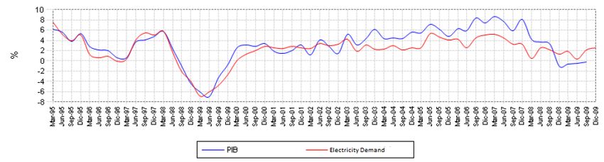
IV Workshop on Modeling and Simulation for Science and Engineering (IV WMSSE) IOP Publishing
Journal of Physics: Conference Series 1938 (2021) 012016 doi:10.1088/1742-6596/1938/1/012016

2. Characteristics of the electricity market

2.1. Fuel price
The long-term prices of fuels are also a reflection of the expectations of the different markets where
different instruments are traded on said assets.

2.2. Hydrological variability
It directly affects markets with a high share of hydroelectric energy, particularly in areas where there
may be strong seasonal and annual differences in tributary flows and reservoirs [6].

2.3. Growth and variability of demand
The acceleration or stagnation in the annual growth rates of electricity demand and the temporary
variability in the energy demand of electrical systems influence prices, market projections and
investment decisions (Figure 1).

Figure 1. Demand growth.

2.4. Modeling and price dynamics
Various behavioral models have been developed that consider the temporary dynamics and volatility of
the prices of these assets. In finance, price processes with uncertainty are modeled with stochastic
differential equations like partial differential equations but with random variables in part of the
equations. The pioneering work in the area is again the article Black and Scholes (1973), which models
the spot price of an action through a process with a single stochastic factor called geometric Brownian
movement.

3. Events of the Colombian electric system

3.1. External events
Nino phenomenon 1997-1998. The warming of the South Pacific produced at the end of 1997 and the
beginning of 1998 a drought of characteristics of strong intensity, considered more intense than those of
the years 1991-1992, although shorter in duration [7]. Hydrology reached 39% from the historical
average for the month of February. This condition produced the highest market prices during the
operation of the market, 249 $ = kWh in September 1997 and 249 $ = kWh in February 1998. This
phenomenon was followed by the opposite Nina phenomenon. The low flow rates at the beginning of
1998 were compensated by the high flows during the rest of the year (in September, the historical
average was 120%), to such an extent that the annual average rose to 90% from the historic. The annual
average was 109% for the year 1999. The reservoir levels recovered, and the use of these reserves was

 2

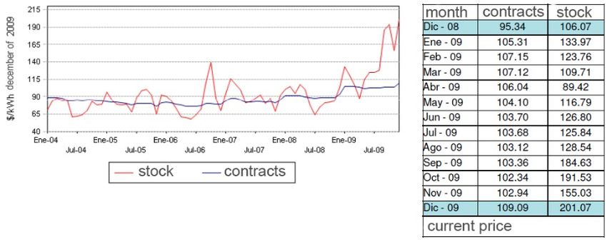
IV Workshop on Modeling and Simulation for Science and Engineering (IV WMSSE) IOP Publishing
Journal of Physics: Conference Series 1938 (2021) 012016 doi:10.1088/1742-6596/1938/1/012016

minimal during the summer of this year, the level fell only to 70% of the total capacity. Stock prices
remained at their low level during the permanence of the phenomenon.

3.2. Characterization of the Colombian electricity system
The energy exchange in Colombia is considered a market of differences in which the operator
determines hour by hour the transactions corresponding to the difference between the purchase
obligations and/or attention to the demand. The formation of the stock price is carried out through a
price auction, in which the generating agents daily and in a single offer block carry out day-ahead price
and availability offers with hourly resolution [8]. From the offers presented by the generators, an
economic dispatch of the energy is made, called ideal dispatch, which determines the available resources
of lower price required to meet the total demand, obtaining as a result the stock price, corresponding to
the price of offer of the generation plant shipped with maximum offer price at the respective time (see
Figure 2 and Table 1).

 • The prices of the contracts are explanatory of the offer. A higher price of contracts increases the
 price of the offer on the stock market, because of valuing the resource more when contracts
 increase in price.
 • Sales on the stock market guide the offer price, especially when they are carried out with equal
 value for all hours of the day, a strategy that corresponds to an optimization of sales on the stock
 market.
 • For some thermal plants, an increase in the supply of the system will lead to an increase in the
 offer price, which is a strategy to induce a higher stock price and maximize income through
 positive reconciliation.

 Table 1. Current price (KW/h).
 Month Contracts Stock
 Dec-08 95.34 106.07
 Jan-09 105.31 133.97
 Feb-09 107.15 123.76
 Mar-09 107.12 109.71
 Apr-09 106.04 89.42
 May-09 104.10 116.79
 Jun-09 103.70 126.80
 Jul-09 103.68 125.84
 Aug-09 103.12 128.54
 Sep-09 103.36 184.63
 Oct-09 102.34 191.53
 Figure 2. Contract variations vs. stock price. Nov-09 102.94 155.03
 Dec-09 109.09 201.07

4. Solution methodology

4.1. Stochastic differential equations
Some physical phenomena can be modelled by means of ordinary differential equations. These are of
the form, Equation (1).

 ẋ = b(x (t)), x (0) = x! , (1)

 whose solution is, Equation (2).

 X (t + Δt) − x (t) = b (bX(t)) + o(Δt). (2)

 3

IV Workshop on Modeling and Simulation for Science and Engineering (IV WMSSE) IOP Publishing
Journal of Physics: Conference Series 1938 (2021) 012016 doi:10.1088/1742-6596/1938/1/012016

 But if we consider the disturbances or noise as “follows”, Equation (3).

 X (t + Δt) − x(t) = b(bX(t)) + “noise” + o(Δt). (3)

 If to the process, we introduce a variable called noise W (t). We will represent a stochastic process
of the form, Equation (4).

 "#
 = b (t,x$ )+σ(t,x$ ) W(t). (4)
 "$

 We will say that W (t) has the following properties.

 • t% ≠ t & if and only if w$% and w$& .
 • {w(t)} is stationary i.e. the joint distribution of {w(t%'$ ),…. w(t ('$ )} It does not depend on t.
 • E [W (t)] = 0 for all t.

 Integral of Ito, given a process X ∈ L& the stochastic integral of X is defined as the continuous
process defined by Equation (5).
 $ $
 I# (t) = ∫! X(u) dW(u) = lim)→+ ∫! X) (u) dW(u) limit in L& . (5)

 So that X) is any succession of simple processes that verify, Equation (6).
 $
 [∫! X) (u) − X(u)& du→ 0 when n→ ∞. (6)

 In the stochastic calculation it would look like this, Equation (7).
 $ $ % $
 ∫! dfw(u) = FUW(t)V − FUW(0)V = ∫! f , (W(u)) dW (u)+& ∫! f ,, (W(u))du. (7)

 Process of Ornstein-Uhlenbeck [9,10], Equation (8).

 Dx(d) = −µX(t)dt + σdw(t) µ, σ > 0. (8)

 To solve the equation, the formula of integration by parts is applied to the process e-$ *X(t) and we
have the Equation (9) [11].

 DUe-$ ∗ X(t)V = e-$ dx(t) + X(t)µe-$ dt + 0 = e-$ (dX(t) + X(t)µdt) = e-$ σdW(t). (9)

 Therefore, the process, Equation (10), solves the stochastic differential equation.
 $
 x(t) = e.-$ x(0) + σe.-$ ∫! e-/ dw(u). (10)

4.2. Time series
Is a chronological series of data under some properties to which information can be extracted
considering that there is a correlation between them that validates our assumption [12,13].

4.2.1. Model autoregressive
A(B) 0 = constant represents a polynomial of delay, for these you have the Equation (11).

 4

IV Workshop on Modeling and Simulation for Science and Engineering (IV WMSSE) IOP Publishing
Journal of Physics: Conference Series 1938 (2021) 012016 doi:10.1088/1742-6596/1938/1/012016

 (1 − ∅% B − ∅& B& − ⋯ … . −∅1 B1 ) z$ = constant + a$ . (11)

 The term autoregressive (AR) can be written as the Equation (12).

 z$ = (1-∅% − ∅& − ⋯ … . −∅1 )µ+∅% z$.% +….∅1 z$.1 +a$ . (12)

 Where we see that it is a linear regression equation, but the dependent variable Z in the period t does
not depend on the values of a certain set of independent variables as it happens in a regression model,
but on its own observed values in periods before t and weighted with the autoregressive coefficients.
[14].

4.2.2. Mobile averages model
The idea is to represent the stochastic process {z$ } whose values can be dependent on each other as a
weighted finite sum of independent random shocks {a$ }, Equation (13) [15].

 ℤ$ = (1- θ% B − θ& B − ⋯ . . θ2 B2 ) a$ = θ(B)a$ . (13)

4.2.3. Model ARMA and ARIMA
A generalization of the AR and mobile averages (MA) models is to combine the models into one and is
known as a model ARMA (p, q), Equation (14).

 φ(B) ℤ$ =θ(B)a$ , (14)

 where φ(B) and θ(B) are order polynomials p and q, {a$ } is a white noise process and ℤ$ is the
series of deviations of the variable ℤ$ with respect to its level µ. The model ARIMA(p, d, q) is the
application of the difference operator to the ARMA model, this is done to eliminate polynomial trends
of order d [16].

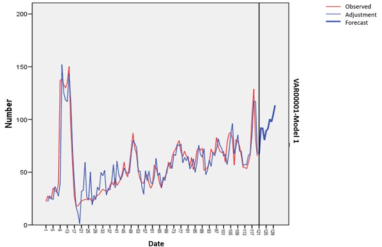
5. Results
Figure 3 shows the energy price (KW/h) in the time window taken (120 data corresponding to 120
months).

 Figure 3. Energy price (KW/h) vs time (months).

5.1. Model with stochastic differential equations
Figure 4 shows the real data (green line) and the first estimate with the Ornstein-Uhlenbeck model (blue
line). The series considered in the Figure 4 takes a very large window of time therefore the estimation
is not appropriate, in the Figure 5 a shorter time window is taken, and it is seen that the estimate improves
but the real data is still insufficient (green line) and the first estimate with the Ornstein-Uhlenbeck model
(blue line).

 5

IV Workshop on Modeling and Simulation for Science and Engineering (IV WMSSE) IOP Publishing
Journal of Physics: Conference Series 1938 (2021) 012016 doi:10.1088/1742-6596/1938/1/012016

 Figure 4. Energy price monitoring.

 Figure 5. Follow-ups at the price of energy different windows of time.

5.2. Model with time series
Figure 6 shows the results using models based on time series (model ARIMA).

 Figure 6. Follow-ups to the price of energy with the time series.

 6

IV Workshop on Modeling and Simulation for Science and Engineering (IV WMSSE) IOP Publishing
Journal of Physics: Conference Series 1938 (2021) 012016 doi:10.1088/1742-6596/1938/1/012016

6. Conclusions
The results based on time series are better than the stochastic equations model, the above does not mean
that the time series are better if and only if idealizations that benefit the technique are used, but in the
case of not having these assumptions stochastic equations are much more adequate. Some alternatives
were explored to estimate the energy price forecast problem, with the aim of reducing the risk for
investors.
 Working with exact techniques is more appropriate when physical considerations are not made on
the problem, otherwise the use of numerical techniques is more appropriate the use of stochastic
equations provides a better understanding of the physical problem and the academic possibility of
investigating more robust solution techniques.

References
[1] Bello S, Beltrán R 2010 Caracterización y pronóstico del precio spot de la energía eléctrica en Colombia
 Revista de la Maestría en Derecho Económico 6 293
[2] Contreras J, Espínola R, Nogales F, Conejo A 2003 ARIMA models to predict next-day electricity prices
 IEEE Transactions on Power Systems 18(3) 1014
[3] Nogales F, Contreras J, Conejo A J, Espinola R 2002 Forecasting next-day electricity prices by time series
 models IEEE Transactions on Power Systems 17(2) 342
[4] Garcia R C, Contreras J, Van Akkeren M, Garcia J B C 2005 A GARCH forecasting model to predict day-
 ahead electricity prices IEEE Transactions on Power Systems 20(2) 867
[5] Conejo A J, Plazas M, Espínola R, Molina A 2005 Day-ahead electricity price forecasting using the wavelet
 transform and ARIMA models IEEE Transactions on Power Systems 20(2) 1035
[6] Lucia J J, Schwartz E S 2002 Electricity prices and power derivatives: evidence from the nordic power
 exchange Review of Derivatives Research 5(1) 5
[7] Schwartz E, J Smith 2000 Short-term variations and long-term dynamics in commodity prices Management
 Science 46(7) 893
[8] V M Guerrero Guzmás 2003 Análisis Estadístico de Series de Tiempo Económicas (Mexico: Thomson)
[9] Oksendal B 2006 Stochastic Differential Equations (Berlin: Springer)
[10] Friedman A 1976 Stochastic Differential Equations and Applications, vol. II (New York: Academic Press)
[11] Black F, Scholes M 1973 The pricing of options and corporate liabilities J. Political Economy 81(1) 637
[12] Alabert A 2004 Introducción a las ecuaciones diferenciales estocásticas (España: Universitat Autónoma
 de Barcelona)
[13] Ito K, McKean H P 1965 Difusion Processes and Their Sample Paths (New York: Springer-Verlag)
[14] William W 1990 Time Series Analysis Univariate and Multivariate Methods (California: Addison Wesley)
[15] Taylor H, Karlin S 1998 An Introduction to Stochastic Modeling (USA: Academic Press)
[16] Botero S, Cano J 2008 Análisis de series de tiempo para la predicción de los precios de la energía en la
 bolsa de Colombia Cuadernos de Economía 27(48) 173

 7