Top 10 Artificial Intelligence Algorithms in Computer Music Composition

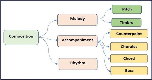
International Journal of Computing and Digital Systems
 ISSN (2210-142X)
 Int. J. Com. Dig. Sys. 10, No.1 (Feb-2021)
 http://dx.doi.org/10.12785/ijcds/100138

 Top 10 Artificial Intelligence Algorithms in Computer
 Music Composition

 Nermin Naguib J. Siphocly1, El-Sayed M. El-Horbaty1 and Abdel-Badeeh M. Salem1

 1Faculty of Computer and Information Sciences, Ain Shams University, Cairo, Egypt

 Received 02 Sep. 2020, Revised 28 Dec. 2020,, Accepted 24 Jan. 2021, Published 8 Feb. 2021

Abstract: Music composition is now appealing to both musicians and non-musicians equally. It branches into various musical tasks
such as the generation of melody, accompaniment, or rhythm. This paper discusses the top ten artificial intelligence algorithms with
applications in computer music composition from 2010 to 2020. We give an analysis of each algorithm and highlight its recent
applications in music composition tasks, shedding the light on its strengths and weaknesses. Our study gives an insight on the most
suitable algorithm for each musical task, such as rule-based systems for music theory representation, case-based reasoning for
capturing previous musical experiences, Markov chains for melody generation, generative grammars for fast composition of musical
pieces that comply to music rules, and linear programming for timbre synthesis. Additionally, there are biologically inspired
algorithms such as: genetic algorithms, and algorithms used by artificial immune systems and artificial neural networks, including
shallow neural networks, deep neural networks, and generative adversarial networks. These relatively new algorithms are currently
heavily used in performing numerous music composition tasks.

Keywords: Computer Music Composition, Machine Learning Techniques, Artificial Intelligence, Music Composition Tasks

 results attracted researchers more to the field of computer
1. INTRODUCTION music composition.
 Thanks to the advancements in computer music Music composition is the task of devising a new
composition, it is of no surprise today to find non- musical piece that contains three main components:
musicians composing very nice music, even on-the-go. melody, accompaniment, and rhythm. Fig. 1 labels the
The desire to compose music with the aid of computers main musical tasks lying under the computer music
returns back to the early days of computer invention. A composition umbrella, further with their types. Melody
common belief is that the first musical notes produced by generation is devising the musical notes pitch; “melody”
a computer were heard in the late 50’s (Illiac Suite) by is the group of consecutive notes forming the musical
Hiller et al. [1] through ILLIAC I computer at the piece while a note “pitch” [5] is the human interpretation
University of Illinois at Urbana–Champaign. However, a of the note’s frequency that distinguishes it from other
recent research by Copland et al. [2] shows that musical notes. Timbre [6], another aspect of the musical piece’s
notes produced from computers were heard even earlier, melody, is defined by the American Standard Association
in the late 40’s, by Alan Turing; the father of modern (ASA) to be “That attribute of sensation in terms of which
computer science himself. Although not intended a listener can judge two sounds having the same loudness
primarily to compose music, Turing emitted repeating and pitch are dissimilar” [7]. Thus, timbre generation
clicks from the loudspeaker of his Manchester computer helps in the interpretation of musical instruments that play
with certain patterns; which were interpreted by human the melody. Music accompaniment has four types:
ears as continuous sound or musical notes. Building on counterpoint, chorales, chord, and bass. Counterpoint [8]
this and using the same Manchester computer, is a special type of music accompaniment that represents
Christopher Strachey, a talented programmer, succeeded the harmony between multiple accompanying voices
in 1951 to develop a program that plays Britain’s national (typically two to four) generated by a set of strict rules.
anthem “God Save the King” [3] along with other Chorale [9] accompaniment is formed of four-part music
melodies, which were then recorded and documented by lines; soprano and three other lower voices. Chord [10]
the BBC [4]. It is still undeniable that Hiller’s research [1]

E-mail: nermine.naguib@cis.asu.edu.eg, shorbaty@cis.asu.edu.eg, absalem@cis.asu.edu.eg
 http://journals.uob.edu.bh

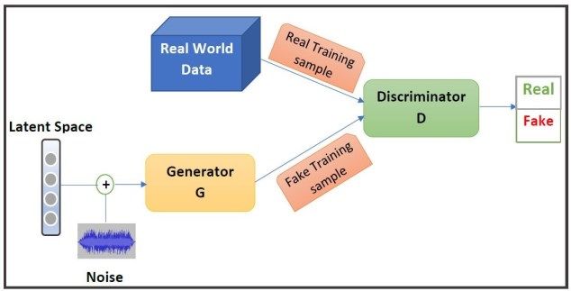
374 Nermin Naguib J. Siphocly, et. al.: Top 10 Artificial Intelligence Algorithms in Computer…

 in this work; such as improvisation (where the computer
 plays on-the-go harmonic music with human players) and
 expressive performance (which is concerned with
 simulating the personal touch of music players).
 The rest of this paper is organized as follows: Sections
 2 to 11 list each of the algorithms under study along with
 their recent applications in computer music composition.
 More specifically: Section 2 describes rule-based systems,
 Section 3 discusses case-based reasoning systems, Section
 4 describes Markov chains generally focusing on the
 Figure 1. Computer Music Composition Tasks hidden Markov model. Section 5 describes generative
accompaniment is a prominent type of harmony where a grammars focusing on the Chomsky hierarchy. Section 6
chord is the group of multiple harmonic notes that sound describes linear programming. Section 7 elaborates on
agreeing when heard. Closely related to chord genetic algorithms. Section 8 discusses artificial immune
accompaniment generation is bassline [11] generation. systems. Sections 9 and 10 cover shallow and deep
Musical piece’s rhythm [12] controls its speed and style; it artificial neural networks respectively. Finally, Section 11
is the beat of the piece. sheds the light on one of the most recent and promising
 Computers can aid, either fully or partially, in each of machine learning techniques used in music composition
the aforementioned musical tasks. Along the years, which is the use of generative adversarial networks. We
research has been carried out for developing algorithms compare the presented algorithms and discuss their merits
that automates each of these musical tasks, which lead to in Section 12. Finally, we conclude our survey in Section
the term “algorithmic composition”. Artificial Intelligence 13.
(AI) had a great share of the research in algorithmic
composition since teaching computer the various music 2. RULE-BASED SYSTEMS
composition tasks needs high levels of creativity. Rule-Based systems (sometimes known as knowledge-
Computer music composition is all about emulating based or expert systems) are means of capturing human
human creativity in music and that specifically is the knowledge in a format comprehensible by computers.
challenge of AI [13]. Rule-based systems mainly aim to aid humans in decision
 The machine learning field is a subset of AI that is making; for example, medical expert systems help doctors
concerned by how computers learn from the given data. in reaching the right diagnosis for patients based on the
Instead of explicitly instructing computers how to perform given symptoms.
tasks step-by-step, machine learning techniques enables 2.1 Overview and Description
computers to interpret relationships from the given data
and accordingly perform tasks such as classification, A rule-based system has three main components:
clustering, regression, and prediction. 1. Knowledge Base (KB): set of IF-THEN rules
 In this paper, we study the top ten AI algorithms used representing the captured knowledge. The IF part
in computer music composition with their applications. of a rule is called antecedent and the THEN part
Also, the most recent machine learning techniques used in is called consequence. The KB might also
music composition for automating the various musical contain facts (known assertions).
tasks are discussed. We first give an overview of each 2. Inference Engine (IE): component responsible for
algorithm; its description, technical background, or inferring or deducing new information from the
pseudocode as needed. Then, we discuss its applications knowledge base according to the system input. It
in the field of music composition. Our main focus is on matches the rules in the knowledge base with the
the applications that have been developed in the last ten current state of the world present in the working
years. We consider very few older papers due to their high
 memory.
impact in the field. Finally, we list the strengths and
weaknesses of each algorithm. Kindly note that we only 3. Working Memory (WM): storage holding
focus on the music composition field; there are other temporary data (assertions) about the current
fields of computer music generation that are not of interest state.

 http://journals.uob.edu.bh

Int. J. Com. Dig. Sys. 10, No.1, 373-394 (Feb-2021) 375

 While TRUE do
 Match Goal with KB
 Find all matches between KB and WM
 if a match is found then
 for each match M do
 return TRUE
 if M does not change WM then
 end if
 Mark M as defunct
 Match Goal with rules consequences
 end if
 if Match(es) is/are found then
 end for
 for each matched rule antecedent A do
 if Number of unmarked matches = 0 then
 TERMINATE Call Backward Chaining(A)
 end if end for
 if Number of unmarked matches > 1 then if all recursive calls return TRUE then
 Call Resolve_Conflict return TRUE
 end if else
 Fire matched rule return FALSE
 Assert rule consequence in WM end if
 end while else
 return FALSE
 Figure 2. Forward Chaining Algorithm end if

 The inference engine can infer data through either
 Figure 3. Backward Chaining Algorithm
forward or backward chaining. Pseudocode of the forward
chaining inference algorithm is listed in Fig. 2. The idea using Derive 6 software which is a computer algebra
behind forward chaining is simply to find all the possible system. Navarro-Cáceres et al. [10], encoded rules about
matches from the knowledge base that are relevant to the chord construction and progression in a penalty function.
current state of the working memory. The forward Then, they employed an Artificial immune system
chaining algorithm then makes sure that a matched rule (discussed in Section 8) to suggest the next chord in a
only fires if its consequences will affect the working given sequence such that this chord minimizes the penalty
memory (change its current state). After marking all the function.
defunct rules; which are rules that will not affect the
working memory, the algorithm will continue only if the 3. CASE-BASED REASONING
number of unmarked matches is not equal to zero. A The most common definition for Case-Based
conflict resolution technique might be needed if there are Reasoning (CBR) is that it is an approach for solving
more than one unmarked match. Conflict resolution helps problems by means of previous experiences. CBR aims
to select only one matched rule to fire. The selected rule for simulating human reasoning and learning from past
then fires, and its consequences are asserted in the experiences. Hence, it is a method of retrieving and
working memory. The process repeats until no more reusing successful solutions from past problems. Unlike
matches will affect the working memory. Forward rule-based systems that keep general knowledge about the
chaining is known as data-driven approach since it starts problem domain, CBR employs the knowledge of
from the already given facts to extract more information. previous solutions for specific problems in the domain.
Thus, it is seen as a bottom-up approach. Moreover, CBR systems keep adding new knowledge
 from learned experiences of newly solved problems.
 On the other hand, backward chaining aims to prove
whether a goal is true or not. Backward chaining 3.1 Overview and Description
pseudocode is listed in Fig. 3. The algorithm first A CBR system keeps information about previous
matches the goal with the knowledge base facts; if a problems in what is called a case base. A “case” has the
match is found, it returns true. If no fact matches the goal, description of a previously solved problem along with its
all rules consequences are checked whether they match solution. The three main operations in the CBR cycle are:
the goal. If the goal does not match any of the rules’ case retrieval, adaptation, and storing. Fig. 4 shows a
consequences, the algorithm returns false. Else, backward diagram for the CBR cycle. When a new problem is
chaining is called recursively on all the matched rules presented to the system, the similar cases to that problem
antecedents keeping track of all the bound variables in the are retrieved from the case base. The next step is to adapt
recursion process. If all the recursive calls return true, the
algorithm is said to succeed and returns true. Backward
chaining is called goal-driven inference approach since it
starts with the goal and searches for a possible match in
the knowledge base, which makes it a top-down approach.
2.2 Rule-Based Systems in Algorithmic Composition
 Rule-based systems are convenient for counterpoint
type of harmony since it is based on rigid rules for
generating harmonic voices. Aguilera et al. [14] coded
 Figure 4. CBR cycle diagram
counterpoint rules with the help of probabilistic logic

 http://journals.uob.edu.bh

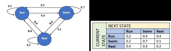
376 Nermin Naguib J. Siphocly, et. al.: Top 10 Artificial Intelligence Algorithms in Computer…

the retrieved cases and their solutions to meet the consists of training the Markov model with the retrieved
demands of the new problem. Finally, the newly solved cases. The adapted case is then evaluated and stored in the
problem is stored in the case base for future retrievals. case base for future retrievals. Within the case adaptation
 phase, their system depended on user feedback to guide
 Design decisions of CBR systems include how to pitches and note duration. Generally speaking, CBR needs
represent the case, which also affects the retrieval quality. external guidance to successfully compose the desirable
Case representation includes mainly some parameters or melodic pieces.
descriptors for the state of the world when the problem
happened accompanied by the solution that worked for 4. MARKOV CHAINS
solving the problem. Another design issue in the retrieval
process is the matching algorithm for comparing the new Before introducing Markov chains, we need to define
problem with the previous cases. The simplest way of stochastic processes and chains. A stochastic process
matching is to apply nearest neighbor between each describes a sequence of events that depend on the time
attribute in the new problem and its corresponding in the parameter t. The set of events is called the “state space”,
current case from the case base, then the cases having the and the set of parameters is called the “parameter space”.
largest weighted sum of all attributes, are retrieved. The Stochastic chain refers to a stochastic process that
case adaptation technique is chosen according to how consists of a sequence of a countable number of states.
close the matched case is to the current problem. 4.1 Overview and Description
3.2 CBR in Algorithmic Composition A Markov chain can be defined as a special case of
 CBR is a very suitable approach for melody stochastic chains in which the probability of a future event
generation systems as these mainly aim to emulate the X(t+1) (random variable X at time t+1) depends on the
experience of human composers. CBR systems give the current state X(t) according to the following equation:
ability to apprehend previous composition experiences to P(Xtm+1 = j|Xtm = i) = pij(tm,tm+1)
be utilized in the generation of new compositions of the
same style. To our knowledge, the recent applications of This expression represents the transition probability of
CBR in music composition are few. Instead, CBR is state Xtm=i at a given time tm to the state Xtm+1=j. A higher
applied extensively in the field of expressive performance order Markov chain is a Markov chain where each state
which is outside the scope of this paper as previously depends on more than one past state such that the order
mentioned. number indicates how many past states affect the current
 state. A Markov chain can be represented as a state
 Ribeiro et al. [15] developed a system that generated transition graph (also known as a Markov state space
melody lines given a chord sequence as an input. Each graph), where each edge shows the transition probability
case in the case-base contains a chord along with its as shown in Fig. 5(a). Note that the sum of all
corresponding melody line and rhythm. Case matching is probabilities on the edges leaving each state is always
through comparing chords based on “Schöenberg’s chart one. Equivalently, a Markov chain can be represented by
of the regions”. The system enables a set of a transition matrix as shown in Fig. 5(b).
transformations to modify the output melody before
adapting the case and storing the produced solution in the Both figures describe the daily sportive activities of a
case base. Navarro-Cáceres et al. [5] developed a system man. He randomly spends his daily workout running or
whose purpose is to assign probabilities for given notes swimming and rests on some other days. By observing his
following the last note of the melody. Their system was sportive patterns, it was found that if he spends his
built upon a CBR architecture accompanied by a Markov workout on a certain day running, it is unlikely to see him
model. The case base holds past solutions and melodies run on the following day (with probability 0.2). Instead, it
and cases are retrieved according to the user’s choices of is more
the desired style, composer, etc. The adaptation step

 Figure 5. (a) Markov state space graph example - (b) Markov transition matrix example

 http://journals.uob.edu.bh

Int. J. Com. Dig. Sys. 10, No.1, 373-394 (Feb-2021) 377

likely to see him either swim or rest on the following day
 forward[i,j] ← 0 for all i,j
(both with an equal probability of 0.4). On the other hand, forward[0,0] ← 1.0
if he spends his workout swimming on a certain day, it is for each time step t do
very probable to see him swim again on the following day for each state s do
(with probability 0.7). It is very unlikely to see him run or for each state transition s to s’ do
rest (with probabilities of 0.2 and 0.1 respectively). After forward[s’,t + 1]+ = forward[s,t] ×
a day of rest, he will probably spend the next day running a(s,s’) × b(s’,ot)
or swimming (both with an equal probability of 0.4). He end for
 end for
will hardly rest the next day (with probability 0.2). end for
 An advanced type of Markov chains is the Hidden return Σforward[s,tfinal+1] for all states s
Markov Model (HMM) that allows us to predict a
sequence of unknown “hidden” variables from a set of
observable variables. That is to say that the set of Notes
observable output symbols of the Markov model are 1. a(s,s’) is the transition probability from state s to s’
visible, but their internal states and transitions are not. 2. b(s’,ot) is the probability of state s’ given observation ot
Each state generates an emission probability. An HMM
represents a coupled stochastic process due to the Figure 6. Forward Algorithm
presence of transition probabilities in addition to the state-
dependent emission probabilities of observable events. viterbi[i,j] ← 0 for all i,j
 viterbi[0,0] ← 1.0
 Any HMM can be formally described by: for each time step t do
 S = S1, S2, ..., SN. Set of N states for each state s do
 for each state transition s to s’ do
 π = π1, π2, ..., πN. Initial state probabilities
 newscore ← viterbi[s,t] ×
 A = aij. The transition probabilities from state i to state j a(s,s’) × b(s’,ot)
 O = o1, o2, ..., oT. The set of T observable outputs if newscore > viterbi[s’,t + 1] then
 belonging to the set of output symbols viterbi[s0,t + 1] ← newscore
 Ot ∈ v1, ..., vM maxscore ← newscore
 B = bit. The probability that observable output end if
 ot is generated from state i save maxscore in a queue
 end for
 end for
 There are three main algorithms for training HMM: end for
1 Forward algorithm: the probability of the observed return queue
 sequence is computed while all parameters are
 known. The opposite to the forward is the backward Notes
 1. a(s,s’) is the transition probability from state s to s’
 algorithms that computes probability in the opposite 0
 2. b(s ,ot) is the probability of state s given observation ot
 ’
 direction.
2 Viterbi algorithm: the most likely sequence of Figure 7. Viterbi Algorithm
 hidden path (Viterbi path) is calculated based on the
 given observable sequence. Initialize HMM Parameters
 Iterations = 0
3 Baum-Welch algorithm: calculates the most likely repeat
 parameters of HMM based on the given observable HMM ′ ← HMM ; Iterations ++
 sequence. for each training data sequence do
 Execute forward algorithm
 Fig. 6, Fig. 7, and Fig. 8 - adapted from [16] - show
 Execute backward algorithm
simple pseudocodes for the aforementioned algorithms.
 Update HMM Parameters
4.2 Markov Chains in Algorithmic Composition end for
 until |HMM − HMM ′ | < delta OR iterations > MAX
 Markov chains have been extensively used in music
composition since the early research attempts in the field.
As previously mentioned, for HMM there is a given set of Figure 8. Baum-Welch Algorithm
observable events and we are to calculate the most
probable states leading to these events. Similarly, in As for the applications of Markov chains in melody
computer music, we have a set of desirable notes pitch generation; as aforementioned in Section 3.2, María
sequence forming a nice musical piece and we try to Navarro-Cáceres et al. [5] combined a Markov model
figure out the possible paths leading to this piece to with case-based reasoning in the adaptation step in order
produce similar pieces in the future. that the Markov model is trained by the retrieved cases to
 predict the successive notes probabilities. Markov models

 http://journals.uob.edu.bh

378 Nermin Naguib J. Siphocly, et. al.: Top 10 Artificial Intelligence Algorithms in Computer…

also aided in counterpoint accompaniment generation. where S refers to “sentence” NP refers to “nominal
Padilla et al. [17] developed a recent emulative system phrase”, VP refers to “verbal phrase”, Det is for article
that generates two-voice counterpoint based on Palestrina- (determiner), Adj is for adjective, N is for noun, and Adv
style. Being trained on limited data, the Markov model is for adverb. Fig. 9 shows the derivation of a sample
was not enough for capturing all the musical features sentence using this generative grammar. The last row of
found in counterpoint. Hence, Padilla’s system worked on the derivation holds the terminal symbols that cannot be
discovering repeated patterns in each piece of the corpus further rewritten in contrast to the non-terminal symbols.
(template) from different viewpoints. The discovered Terminal symbols (in our example: The, scared, boy,
patterns were then fed into the Markov model for runs, and furiously) are to be found in the language
generating a two-voice counterpoint in terms of those lexicon.
patterns.
 Noam Chomsky [19] classified generative grammars
 Wassermann and Glickman [18] have recently into four types according to their restriction level from
developed two novel approaches for harmonizing chorales type-0 (unrestricted) to type-3 (highly restricted). This
in Bach style. In the first approach, the primary input into classification is now known as “the Chomsky hierarchy”.
a chorale-harmonization algorithm is the bass line, as
opposed to the main melody. Their second approach Fig. 10 shows a visual representation of the Chomsky
combines music theory and machine-learning techniques hierarchy. From the figure it is clear that each type is
in guiding the harmonization process. They employ a contained in the less restrictive types. In other words, a
hidden Markov model in learning the harmonic structure type-3 grammar is also a type-2, a type-1, and a type-0
and apply a Boltzmann pseudolikelihood function grammar. Similarly, a type-2 grammar is also a type-1 and
optimization for determining individual voice lines. They a type-0 grammar.
incorporate musical constraints through a weighted linear Table 1 compares the four types of grammars defined
combination of constraint indicators. They evaluated their by Chomsky. As we go down in the Chomsky hierarchy
model through a group of test subjects who could not (from type-0 to type-3), complexity and generative
easily distinguish between the generated chorales and the capacity decrease while restrictions increase. Type-0
original Bach chorales. The bass-up approach grammars produce the recursively enumerable languages
outperformed the traditional melody-down approach in recognized by a Turing machine. It has the lowest level of
out-of-sample performance. restriction and the highest generative capacity.
5. GENERATIVE GRAMMARS Deciding whether a string belongs to such a language
 is an undecidable problem. The rules of type-0 grammars
 Language, in its simplest definition, is a set of symbol
 are in the form: α →β such that α and β are any sets of
strings (sentences) whose structure abides to certain rules.
 terminal and non-terminal variables.
A formal language is that provided with mathematical
description of both its alphabet symbols and formation Type-1 grammars define context-sensitive languages.
rules. A grammar describes how a sentence is formed and In this case, the number of symbols on the left-hand side
distinguishes between well-formed (grammatical) and ill- of a rule must be less than or equal to the number of those
formed (nongrammatical) sentences. A generative on its right-hand side. Type-1 grammars are also highly
grammar is a recursive rule system describing the generative, of exponential complexity, and recognized by
generation of well-formed sentences (expressions) for a linear bounded automata. Type-2 grammars, on the other
given language. String sequences in a generative grammar hand, describe context-free languages that are recognized
are formed through rewriting rules where symbols on the by pushdown automata which can make use of stack in
right-hand side replace symbols on the left-hand side of a determining a transition path. They are of medium
rule. generative capacity and of polynomial complexity.
 Finally, Type-3 grammars or regular grammars are the
5.1 Overview and Description least generative and the most restrictive of all the four
 In the following we give an example of generative types. Its rules are restricted to only one non-terminal on
grammar which can be used to derive a simple English the left-hand side and only one terminal on the right-hand
sentence. The grammar rules are as follows: side possibly followed by a non-terminal. Type-3
 S → NP VP grammars are of linear complexity and is recognized by
 deterministic or non-deterministic finite state automata
 NP → Det NP (DFA or NFA).
 NP → Adj N
 VP → V Adv

 http://journals.uob.edu.bh

Int. J. Com. Dig. Sys. 10, No.1, 373-394 (Feb-2021) 379

 Figure 9. Derivation of a generative grammar
 On the other hand, a renowned grammar system is Figure 10 - Chomsky Hierarchy
Lindenmayer System or L-System [20] which is famous Hamanaka et al. [22] is an example of the works inspired
for parallel rewriting. Parallel rewriting is finding all the by the book.
possible derivations for a given rule simultaneously.
These are especially suited for representing self-similarity. Cruz-Alcázar et al. [23] developed a grammatical
L-Systems were used primarily in microbial, fungal, and inference system for modeling a musical style which was
plant growth portrayal. then used in generating automatic compositions. They
 expanded on their work in [24] adding more comparisons
5.2 Generative Grammar in Algorithmic Composition between different inference techniques and music coding
 Forming music through grammars can be achieved by schemes (absolute pitch, relative pitch, melody contour,
replacing strings with music elements such as chords, and relative to tonal center).
notes pitch, and duration. The major design concern in
 A basic approach for employing L-Systems in music
composing music with grammars is the formulation of the
 composition applications was to interpret the graphical
set of grammar rules itself, most of the time this step is
 representations produced by L-Systems into musical notes
carried out manually then rules are fed into the system.
 such as in [25]. Kaliakatsos-Papakostas et.al. [12]
However, there exists other software where grammar rules
 modified finite L-Systems to generate rhythm sequences.
are extracted (inferred) from a previously composed
 Quick and Hudak [26] presented a novel category of
music corpus; a process that is called “grammatical
 generative grammars in their work called Probabilistic
inference”. During the music composition process, a
 Temporal Graph Grammars (PTGGs), that handles the
human composer converges from the main piece theme
 temporal aspects of music and repetitive musical phrases.
towards its individual elements and notes. Likewise,
 Melkonian [27] expanded on Quick and Hudak's [26]
music composition by grammar converges from level to
 probabilistic temporal graph grammars in order to include
level in conjunction with the derivation of symbols and
 generating of melody and rhythm in addition to generating
musical elements.
 harmonic structures.
 One early work that extremely influenced music
composition by grammars, is the book named “A 6. LINEAR PROGRAMMING
Generative Theory of Tonal Music” [21]. The book Linear programming or linear optimization is a subset
describes the relation between tonal music and linguistics of mathematical programming (optimization) where an
where the authors grammatically analyze tonal music. The optimal solution is found for a problem with multiple
book was not intended for computer music composition, decisions about limited resources. In linear programming,
nonetheless, the concepts within the book were further a problem is formulated as a mathematical model with
utilized in this research field. Melody morphing by
 TABLE 1. COMPARISON OF GENERATIVE GRAMMARS

 Generative
 Type Language Automaton Complexity Production Rule
 Capacity
 Recursively
 Type-0 Turing machine Undecidable Very high α→β
 enumerable
 Linear-bounded
 Type-1 Context sensitive Exponential High αAβ → αγβ
 automaton
 Push-down
 Type-2 Context-free Polynomial Medium A→γ
 automaton
 Type-3 Regular DFA or NFA Linear Low A → b or A → bC

 http://journals.uob.edu.bh

380 Nermin Naguib J. Siphocly, et. al.: Top 10 Artificial Intelligence Algorithms in Computer…

linear relationships. Locate a starting extreme point EP
 while TRUE do
6.1 Overview and Description for all the edges containing EP do
 In order to solve a problem using linear programming find the edge E that provides the greatest
the following steps are involved: rate of increase for the objective function
 1. Modeling the problem mathematically end for
 if E = NULL then
 2. Examining all the possible solutions for the RETURN EP % no more increasing edges found
 problem end if
 3. Finding the best (optimal) solution out of all the Move along E to reach the next extreme point
 if a new extreme point is found EP(new) then
 possible ones
 Let BFS = BFS(new)
 A linear programming model can be described as else
follows: RETURN FAIL % The edge is infinite;
 1. Set of decision variables X = {x1,x2,...,xn} no solution found
 2. Objective function Z = c1x1 + c2x2 + ... + cnxn or end if
 end while
 Z = ∑ =1 
 3. Set of constraints: Figure 12. Simplex Algorithm (Basic version)

 a x + a x + ... + a x ≤ b
 11 1 12 2 1n n 1 However, when there are more than two decision
 a x + a x + ... + a x ≤ b
 21 1 22 2 2n n 2 variables, the “simplex method” is adopted for finding the
 . problem solution. Instead of exploring all the feasible
 . solutions, the simplex method deals only with a specific
 . set of points called the “extreme points” which represents
 a x + a x + ... + a x ≤ bm ,
 m1 1 m2 2 mn n
 the vertex points of the convex feasible region containing
 all the possible solutions. Fig. 12 is a basic version of the
 where all elements in X ≥ 0 simplex method described geometrically, for more
 Finding a solution for a two-variable linear mathematical details please check [28] (P. 864 - 878).
programming model is simple; it can be solved The simplex algorithm starts by locating an extreme
graphically via drawing straight lines that correspond to point in the feasible region. Among all the edges
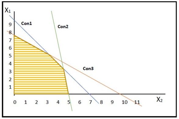
each constraint in a two-dimensional space. The area connected to the extreme point, the algorithm searches for
covered by each straight line contains the values of its the edge with the highest rate of increase in favor of the
possible solutions and the area covered by all the lines objective function. It then moves along this edge until it
(area of intersection) represents the “feasible region” or reaches the next extreme point. The aforementioned step
“feasible solution space”. The shaded area in the graph in might have two results; either a new extreme point is
Fig. 11 is an example of a feasible region; where Con1, found, or the edge turns out to be infinite which means
Con2, and Con3 model the linear equations of each that this problem is unbound and has no solution. This
constraint. algorithm repeats until no more increasing edges are
 found.
 6.2 Linear Programming in Algorithmic Composition
 Linear programming has been excessively employed
 in timbral synthesis; the main idea is to distribute sounds
 in what is called a timbral space. When the user enters
 specific descriptors to describe the desired timbre
 properties, these descriptors are given numerical values
 and represented as linear equations in the timbral space.
 The generated linear equations represent the boundaries of
 the region containing the desired timbre, hence, solving
 them using linear programming results in the optimal
 sound.
 Figure 11. Graph of Linear Programming Model for a Two
 Decision Variables Problem

 http://journals.uob.edu.bh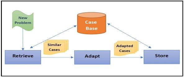

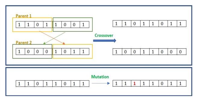
Int. J. Com. Dig. Sys. 10, No.1, 373-394 (Feb-2021) 381

 Timbral synthesis has earlier been based on verbal
 Represent chromosomes in binary format
descriptions. However, Mintz [29] built his timbral Set Size of population to N
synthesis on a more standard format which is MPEG-7. In Set mutation probability to Pm
his method, users can define the timbre they want using Set crossover probability to Pc
standardized descriptors. His model contains a timbral Define the fitness function: Fitness_Fn()
synthesis engine that turns these descriptor values into Produce the first generation of chromosomes
control envelopes producing synthesis equations. The X1,X2,...,XN
coefficients of these equations are mapped as specific repeat
points in the timbral space. Seago et al. [6] also worked for each i do
 Call Fitness Fn(i) to GET the fitness ratio FX
with timbral spaces. They proposed a timbre space search end for
strategy, based on Weighted Centroid Localization repeat
(WCL). They expanded on their work in [30]. However, Choose a pair of chromosomes Xi and Xj
the authors pointed out that this method suffers from slow according to their fitness ratios FX1 and FX2
convergence. Apply genetic operators on Xi and Xj according
 to Pc and Pm
 7. GENETIC ALGORITHMS Add new Xi’ and Xj’ to the new generation
 until number of chromosomes of the new
 Genetic Algorithms (GAs) are a class of evolutionary generation = N
algorithms, they are also considered as stochastic search Replace old generation with the new one
techniques. GAs tend to emulate the natural system of until a chromosome with satisfying fitness is
evolution on computers. Natural evolution is based on the found or the maximum number of generations
fact that organisms produce excess offspring than that is reached
could survive. The large offspring compete over limited
 Figure 13. The Genetic Algorithm
resources; thus, only those individuals who are best suited
to their environment (best fit) will be able to survive. The
surviving offspring reproduces and transfers its traits to its
offspring creating a more fit generation each time.
7.1 Overview and Description
 GAs portray natural evolution by working on a
population of artificial chromosomes. Each artificial
chromosome is formed of a number of genes, each is
represented by a “0” or “1”. Hence, mapping any problem
to be solved by GAs involves, first, encoding individuals
(representing potential solutions) into chromosomes. A
fitness function decides how fit the individuals in each Figure 14. Examples on mutation and crossover
generation are. Genetic operations (crossover and
mutation) on the best fit chromosomes evolve a new Other than selection, a GA mainly relies on the
generation. crossover and mutation operators. Mutation is the
 The steps of GA are demonstrated in more detail in flipping of one randomly selected gene in the
Fig. 13. The very first step is to formulate chromosomes’ chromosome, while crossover involves splitting a pair of
binary genes. The population size is defined from the chromosomes at a randomly selected crossover point and
beginning, same for the crossover and mutation exchange the resulting chromosome sections. Fig. 14
probabilities, Pc and Pm respectively. These probabilities gives an example of each operation.
determine the applied ratio of the crossover and mutation 7.2 GAs in Algorithmic Composition
operations in each generation. A fitness function is then
defined according to the satisfying criteria of describing a GAs have been broadly used in the field of
“fit” chromosome. Next, one generation of chromosomes algorithmic composition. GAs are suited for music
is generated (the first generation). The fitness function is composition applications due to the following [31]:
then applied to each chromosome to return its fitness 1. They help in generating many segments
ratio. According to the returned fitness ratios, the best fit (generations) to form larger musical pieces.
chromosomes are selected, and genetic operators are
 2. Musical segments are continuously generated and
applied to each pair of them. The result is a new
generation of chromosomes that passes through the same examined, which generally complies with the
process over and over again until the desired fitness is composition process and concepts.
attained or until the maximum number of generations is 3. The generated music is always evaluated through
reached. fitness metrics which improves the quality of the
 generated music.

 http://journals.uob.edu.bh

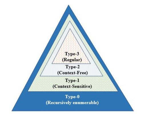
382 Nermin Naguib J. Siphocly, et. al.: Top 10 Artificial Intelligence Algorithms in Computer…

 TABLE 2. COMPARISON BETWEEN ABSOLUTE AND RELATIVE multi-objective fitness function. Moreover, they proposed
 PITCH a new data structure; “Melodic Trees” for chromosomes
 representation. For the task of timbre synthesis, Carpentier
 Absolute Pitch Relative Pitch et al. [33] developed an evolutionary algorithm that, not
 When a chromosome is When a chromosome is only discovers optimal orchestration solutions, but also
 modified the following changed all the following indulges in the examination of non-spontaneous mixtures
 sequence stays intact. notes are affected. of sounds.
 Preferred if transpositions Allows for transposition for GAs were also employed in chord generation, such as
 apply to one voice of whole segment. the polyphonic accompaniment generation (formed of
 polyphonic movement. main, bass, and chord) system of Liu et al. [34]. In their
 Mutation produces larger Mutation causes less system they implemented a fitness function that is built
 modification. modification. upon evaluation rules inspired by music theory. Later,
 4. The generated results are also affected by how they enhanced their system in [35] by mining and
 music is encoded. extracting chord patterns from specific composer’s music
 to be introduced as genes in the GA. In addition to chords,
 Music is encoded either in the form of absolute or Liu’s work included bassline and rhythm generation,
relative pitch; absolute pitch encoding specifies the through the merging of GAs and data mining.
concrete note pitch value in binary, while relative pith
encodes the distance between two consecutive notes. Recently, R. De Prisco et al. [36] developed an
Table 2 compares between absolute and relative pitch. algorithm for automatic music composition using an
 evolutionary algorithm. They work on chorales of four
 Genetic operators are twisted to be applied to music; voices. Their algorithm takes one of the voices as input
for example, mutation and crossover are changed into and produce the rest of the four voices as output. they aim
mirror and crab. However, these twists can be applied to to finding both; suitable chords, in addition to the melodic
western music only where the distance between notes in lines. They not only proposed a novel representation for
the scale are constant. These transformations, on the other the chromosomes, but also, they enhanced the quality of
hand, are supposed to work on musical segments the new generations through customizing operators to
primarily musically related. This is, nonetheless, make use of music theory and musical statistical analysis
problematic in GAs due to the continuous generation of on a Bach’s chorales corpus. As for the fitness function,
new fragments through rearranging chromosomes, and the authors used a multi-objective fitness function dealing
thus, losing their musical structure in the process. Large with both the harmonic and the melodic aspects.
musical fragments are problematic because the musical
context is completely changed with every genetic Abu Doush and Sawalha [37] combined GAs and
operator, resulting in a possibly undesirable abrupt neural networks for composing music. They implemented
modulation. To overcome this issue, we can use rule- a GA to generate random notes and used neural networks
based techniques to control and guide the operators as the fitness function for that algorithm. The authors
according to the musical domain modeled in the rules. compared between four GAs with different combinations
Moreover, since we are dealing with context-dependent of parameters such as; tournament and roulette-wheel for
information, Markov chains and generative grammars can the selection phase and one-point and two-point
be used as promising potential aids to GAs for better crossovers. Their experiments showed that using
handling such information. tournament selection and two-point crossover generate
 music compositions of higher quality.
 Fitness evaluation also represents a challenge for GAs
in music. At first, human user evaluation has been 8. ARTIFICIAL IMMUNE SYSTEMS
adopted for GAs; this however, caused the algorithm to be Researchers developed Artificial Immune Systems
delayed waiting for the user input. Consequently, (AIS) aspiring to find solutions for their research
techniques such as rule-based and neural networks were problems based on concepts inspired by the biological
utilized in fitness functions as a weak alternative to human immune system. The biological immune system protects
evaluation. Nonetheless, research involving more than one our bodies from pathogen attacks (harmful
fitness function proved to produce better results. microorganisms that stimulate immune response). Unlike
 There are plenty of applications of GAs in the the centralization of the neural system that is controlled by
different music composition tasks. As for melody the brain, the biological immune system is decentralized
generation, the work of Pedro J. Ponce de León et al. [32] and distributed throughout the body.
enhanced the selection process through developing a

 http://journals.uob.edu.bh

Int. J. Com. Dig. Sys. 10, No.1, 373-394 (Feb-2021) 383

 The immune system has the advantage of being
robust, self-organized, and adaptive. It has pattern- input: S = a set of antigens, representing data
recognition and anomalies detection capabilities, and it elements to be recognized.
keeps track of previous attacks for better future responses. output: M = set of memory B-cells capable of
When a body is attacked by pathogens, the immune classifying unseen data elements.
system detects them and instantiates a primary defense Generate set of random specificity B-cells B.
 for all antigens ag ∈ S do
response. If the attack repeats later, the immune system
 Calculate affinity of all B-cells b ∈ B with ag.
remembers that past experience and consequently
 Select highest affinity B-cells, perform
launches a secondary response quicker than the primary affinity proportional cloning, place clones
one. The immune system has the ability to differentiate in C.
between self (those belong to the body) and non-self cells for all B-cell clones c ∈ C do
(invaders). The term “B cell” refers to a part of the Mutate c at rate inversely proportional to
immune system that produces antibodies targeting the affinity.
pathogens to be diminished from the body. Antibodies are Determine affinity of c with ag.
produced when B cells clone and mutate after a process of end for
recognition and stimulation. Copy all c ∈ C into B.
 Copy the highest affinity clones c ∈ C into
8.1 Overview and Description memory set M.
 Prior to solving problems by AIS, the “antigens” and Replace lowest affinity B-cells b ∈ B with
 randomly generated alternatives.
“antibodies” need to be defined in terms of the problem end for
domain, and then encoded in binary format. An important
design choice is the “affinity metric” (also called the Figure 16. Clonal Selection Algorithm (Reproduced from [39])
“matching function”) which is pretty similar to the
“fitness function” in GAs. Selection and mutation
 “negative selection” and “clonal selection” algorithms.
operations also need to be determined (mutation is also
 The negative selection algorithm proposed by Forrest et
very similar to that in GAs, based on flipping bits). When
 al. [38], is shown in Fig. 15 reproduced from [39]. Its
all the above is well defined the algorithm can then be
executed. idea is to differentiate between self and non-self cells and
 to react differently to them. The input to this algorithm is
 The most famous selection algorithms in AIS are a set of self strings that are stored and marked as friendly
 normal data. The first phase of the algorithm is the
input: S = set of self strings characterizing generation of string detectors. Detectors are generated as
 friendly, normal data. random strings and matched with the list of self strings
output: A = Stream of non-self strings detected. keeping only those that do not match. The second phase is
Create empty set of detector strings D. to monitor the system for detection through continuously
Generate random strings C. matching the input strings with the detector strings and
for all random strings c ∈ C do streaming out those that match.
 for all self strings s ∈ S do
 if c matches s then Clonal selection is based on the idea of cloning the B
 Discard c cells that are proved to be of the highest match with the
 else antigens (highest affinity). The cloned B cells act as an
 Place c in D
 army for defending the body against antigens; because
 end if
 end for they have the correct antibodies inside them. The clonal
end for selection algorithm is shown in Fig. 16 reproduced from
while there exist protected strings p to check do [39]. The first step in the algorithm is to generate a
 Retrieve protected string p random group of B cells. The affinity is then calculated
 for all detector strings d ∈ D do between each antigen and all the B cells. The B cells of
 if p matches d then the highest affinity are cloned proportionally to the
 Place p in A and output. affinity measure. The cloned cells are mutated with a
 end if probability that is inversely proportional to the affinity
 end for
end while
 measure. The affinity of the mutated clones, with respect
 to the antigen, is then calculated. The B cell clones of
 higher affinity replace the B cells of lower affinity in the
 Figure 15. Negative Selection Algorithm (Reproduced from [39])
 old generation. Furthermore, a copy of the clones with the
 highest affinity is kept in memory.

 http://journals.uob.edu.bh

384 Nermin Naguib J. Siphocly, et. al.: Top 10 Artificial Intelligence Algorithms in Computer…

8.2 AIS in Algorithmic Composition
 As previously mentioned in Section 2.2, AIS has been
used for chord generation by Navarro-Cáceres et al. [10]
to provide a recommendation for the following chord in a
sequence. AIS is unique in that it provides more than one
suggested solution (chord) because multiple optima are
found in parallel. In the case of chord generation, the
suggested multiple optima need to be filtered to offer a
threshold for generating the good chords only. Navarro- Figure 17. Artificial neuron (Adapted from [43])
Cáceres et al. expanded on their work in [40] and
enhanced their AIS so as to optimize an objective function Axon, and Synapses. Dendrites help the neuron receive
that encodes musical properties of the chords as distances information from other neurons. Soma is the cell body
in the so called Tonal Interval Space (TIS). Chord that is responsible for information processing. A neuron
selection is viewed as a search problem in a the TIS sends information through Axon. Synapses help a neuron
geometric space in which all chords are represented under to connect with other neurons in the network.
certain constraints. Navarro-Cáceres’ work is centered
about generating the next candidate chord given the 9.1 Overview and Description
previous two chords as an input; thus, their system An Artificial Neuron (AN) models the biological
captures short-term dependencies only and need neuron; it also has inputs, a node (body), weights
enhancements to generate a chord that depends on the (interconnections) and an output. Fig. 17 adapted from
whole music context rather than the previous few chords [43] shows a diagram of an artificial neural.
only.
 The variables in the figure are:
 For the task of computer aided orchestration, Caetano
et al. [41] developed a multi-modal AIS that comes up 1. Input variables {x1,x2,...,xN}: features or attributes
with new combinations of musical instrument sounds as coming from other neurons connected to the current
close as possible to the encoded sound in a penalty neuron.
function. In contrary to chord generation, the nature of the 2. Weights {w1,w2,...,wN} : factors multiplied by the
orchestration problem is that it may hold more than one inputs to control how much each input is affecting
possibility, hence the aim of Marcelo’s system was to the result.
maximize the diversity in the solution set of the multi-
 3. Summation result a: It is the weighted sum of all
modal optimization problem. This approach led to the
existence of various orchestrations for the same reference inputs.
sound and actually embraced the multiple optima 4. Bias b: A constant affecting the activation function
phenomena in AIS. f(u) where = + = ∑ =1 + 
 5. Error threshold θ = -b which is applied to the neuron
 Navarro‑Cáceres et al. [42] have recently introduced
an interesting application for chords generation based on a output to decide whether the neuron will fire or not.
neurological phenomenon called Synesthesia. In this 6. Neuron output Y = f(u)
phenomenon, the stimulation of one sensory, results in 7. Activation Function f(u): It is the function applied to
automatic, involuntary experiences in a second sensory. u to determine the final output Y. f can be a linear,
Inspired by this phenomenon, the authors extract sound step, or sigmoid function, among others.
from colors for chord progressions generation utilizing an One of the building blocks of neural networks design
AIS. They extract the main colors from a given image and is the “network topology” which is how the neurons are
feed them as parameters to the AIS. They developed an organized in the network. There are two main types of
optimization function to come up with best candidate topology:
chord for the progression, according to its consonance and
relationship with the key and the previous chords in the 1. Feedforward networks: In a feedforward network
progression. signals move in one direction from input to output. A
 feedforward network can either be:
 9. ARTIFICIAL NEURAL NETWORKS (a) A single layer feedforward network (single layer
 Artificial Neural Networks (ANNs) aim for simulating perceptron): A network having only one layer of
the biological neural system controlled by the brain. A nodes connected to the input layer. This type of
biological neural system is composed of small network is typically used to solve linearly
interconnected units called neural cells or neurons. A separable classification problems.
biological neuron is a special type of cells that processes
information. A neuron has four parts: Dendrites, Soma,

 http://journals.uob.edu.bh

Int. J. Com. Dig. Sys. 10, No.1, 373-394 (Feb-2021) 385

 (b) A multilayer feedforward network: A network
 Initialize weights (small random values)
 having one or more layers between the input and
 repeat
 the output layer. Multilayer networks are fully for each training sample do
 connected which means that each neuron in one
 –FEEDFORWARD–
 layer is connected to all the neurons in the next
 layer. This type of networks is typically used to Each input unit receives an input signal Xi
 solve non-linearly separable classification ∈ {x1,x2,...,xn} and broadcasts it to all
 the hidden units in the next layer
 problems.
 Each hidden unit Zj ∈ {Z1,Z2,...,Zp} sums the
2. Feedback Networks: In a feedback network signals weighted input signals:
 can flow in both directions such as in the case of
 _ = 0 + ∑ni=1 x 
 Recurrent Neural Networks (RNNs) which have
 then applies the activation function to the
 closed loops in their architecture. They have output zi = f(z_inj) then broadcast its
 connections from units in a layer leading to the same signal to all the units in the output layer
 layer or to previous ones through what is called Each output unit Yk ∈ {y1,y2,...,ym} sums the
 “context neurons”. This kind of networks is dynamic weighted input signals:
 and keeps changing until it reaches an equilibrium p
 _ = 0 + ∑j=1 z 
 state. RNNs provide a means of storing information then applies the activation function to
 from previous epochs (training cycles) and using the
 them in future ones, i.e. they support long-term output = ( _ )
 dependencies. For even more support of long-term
 –BACKPROPAGATION–
 dependencies, Long Short-Term Memory (LSTM)
 networks add memory block units to recurrent For each output unit Yk ∈ {y1,y2,...,ym}, the
 error σk is computed between the output
 networks.
 signal and the target sample corresponding
 ANNs are trained (they learn) to perform the desired to the
tasks. There are three ways an ANN can learn with: training input sample

 1. Supervised learning: A dependent type of = ( − ) ′( _ )
 where f0 is the derivative of the
 learning in which the output of the network is
 activation function. The weight correction
 compared with the desired output. According to term is then
 the difference between the actual output and the calculated
 desired output, the weights of the network are
 ∆ = 
 updated until the neuron’s output match the target and the error σk is transferred to all the
 output. Supervised learning examples include: hidden units in the previous layer
 the delta rule for training single layer perceptrons For each hidden unit Zj ∈ z1,z2,...,zp the
 and the backpropagation algorithm to train weighted sum of the transferred error is
 multilayer networks. calculated
 2. Unsupervised learning: An independent type of _ = ∑ 
 =1 
 The error information is then calculated:
 learning typically used for clustering input data
 of similar types or for dimensionality reduction. = _ ′( _ )
 3. Reinforcement learning: A semi-dependent type and the weight correction term is
 of learning based on reward and punishment. calculated:
 Without labeled data items, the network receives where α is the
 ∆ = 
 a feedback from the environment as an evaluation Learning rate
 to its performance. Weights of the hidden layer are updated

 Since backpropagation is one of the most powerful ( ) = ( ) + ∆ 
learning algorithms that are widely used in different types Weights of the output layer are updated
of ANNs, we provide a simplified version of this
 ( ) = ( ) + ∆ 
algorithm in Fig. 18 (adapted from [44]), assuming the
network has only one hidden layer. The input training end for
samples (or vectors) are fed into the network and until Error threshold is reached
transferred to the hidden layer as weighted sums. The
hidden layer units apply an activation function to these
sums, then they transfer the results to the output layer Figure 18. Backpropagation Algorithm (Adapted from [44])
units as another set of weighted sums. The output of the

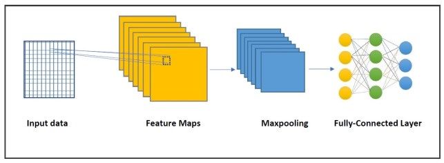
 http://journals.uob.edu.bh

386 Nermin Naguib J. Siphocly, et. al.: Top 10 Artificial Intelligence Algorithms in Computer…

network is the result of applying the activation function in
the output layer. The difference between the output and
the corresponding target sample data is calculated which
serves as the error factor. The weighted error sum is
propagated backward from the output layer to the hidden
layer and from the hidden layer to the input layer.
Meanwhile, the weight correction factor is calculated for
each unit (in terms of the error factor) which is then used
to update the network weights. The whole process is Figure 19. Convolutional Neural Network Architecture
repeated until the error becomes less than a given (Adapted from [48])
threshold.
 convolution layer in a CNN applies several filters on the
9.2 ANNs in Algorithmic Composition input data such that each filter extracts a specific feature
 There are many examples of using ANNs in musical from it. The maxpooling layer performs dimension
tasks. For chorale music, Hadjeres et al. [45] aimed for reduction by keeping only data items of highest values
imitating Bach’s chorales in their system using a within the pooling size. The output from maxpooling is
dependency network and pseudo-Gibbs for the music then flattened to be introduced to a fully connected neural
sampling. On the other hand, Yamada et al. [9] set up a network which in turn produces the final output.
comparison between adopting Bayesian Networks (BNs) The convolutional layer performs the computation
and recurrent neural networks in chorale music generation defined by the following mathematical equation (the dot
to show the strengths and weaknesses of each. product between the input data and a given filter):
 Recent research about chord generation using ANNs ( ∗ )( , ) = ∑ +ℎ + 
 = −ℎ ∑ = − ( , ) ( − , − )
include that of Brunner et al. [46] and of Nadeem et al.
[47]. The former’s system produces polyphonic music where I is the input, F is the filter of width 2w + 1 and
based on combining two LSTMs. The first LSTM height 2h + 1. F is defined over [−w,w] × [−h,h]. A simple
network is responsible for chord progression prediction pseudocode for the convolution process is described in
based on a chord embedding. The second LSTM then uses Fig. 20 adapted from [49]. This can be interpreted
the predicted chord progression for generating polyphonic visually as a window scanning the input data from left to
music. The latter’s system produces musical notes right and from up to down moving one cell at a time. At
accompanied by their chords concurrently. They use a each step, a dot product is computed between the
fixed time-step with a view to improve the quality of the window’s values and the current values of the input data
music generated. To produce new music, chords and notes that corresponds in position to the window. These steps
networks are trained in parallel and afterwards their repeat until the algorithm finishes scanning the input data.
outputs are combined through a dense layer followed by a Training the CNN can be done through applying the
final LSTM layer. This technique ensures that both inputs, backpropagation algorithm on the features map produced
notes and chords, are being dealt with along all the steps from the convolution process in the fully-connected layer.
of generation, and thus, become closely related. As
mentioned earlier in Section 7.2, Abu Doush and Sawalha 10.2 DNNs in Algorithmic Composition
[37] employed neural networks to compute the fitness
function for a GA. They were trained to learn the Given the filter array F of size Fw ×Fh and the
regularity and patterns of a set of melodies. input data array I of size Iw × Ih
 for y from 0 to Ih do
 10. DEEP NEURAL NETWORKS for x from 0 to Iw
 do sum = 0
 Deep Neural Networks (DNNs) are distinguished from for j from 0 to Fh do
single hidden layer ANNs by their depth. The network’s for i from 0 to Fw do
depth means the number of layers that an input has to pass
 sum += I[y + j][x + i] ∗
through until it reaches the output layer.
 F[j][i]
10.1 Overview and Description end for
 end for
 A famous type of deep neural networks is the
 C[y][x] = sum/(Fw ∗ Fh)
Convolutional Neural Network (CNN). CNNs apply the
 end for
convolution operation instead of general matrix
 end for
multiplication (weighted sum) in at least one of its layers.
 return C
Fig. 19, adapted from [48], shows the general architecture
of a CNN. The main building blocks of a CNN are the
input, output, convolutional, pooling, and fully connected
 Figure 20. Convolution Pseudocode (Adapted from [49])
layers. The idea behind CNNs is to decompose a given
problem into smaller ones and work on solving each. the

 http://journals.uob.edu.bh