Tutorial on UAVs: A Blue Sky View on Wireless Communication - arXiv.org
←
→
Page content transcription
If your browser does not render page correctly, please read the page content below
TUTORIAL ON UAVS: A BLUE SKY VIEW ON WIRELESS COMMUNICATION                                                                     1

                                          Tutorial on UAVs: A Blue Sky View on Wireless
                                                         Communication
                                        Evgenii Vinogradov*, Hazem Sallouha, Sibren De Bast, Mohammad Mahdi Azari, Sofie
                                                                              Pollin

                                                                                                    Abstract
                                                  The growing use of Unmanned Aerial Vehicles (UAVs) for various applications requires ubiquitous and reliable
arXiv:1901.02306v1 [cs.NI] 8 Jan 2019

                                             connectivity for safe control and data exchange between these devices and ground terminals. Depending on the
                                             application, UAV-mounted wireless equipment can either be an aerial user equipment (AUE) that co-exists with
                                             the terrestrial users, or it can be a part of wireless infrastructure providing a range of services to the ground users.
                                             For instance, AUE can be used for real-time search and rescue and/or video streaming (surveillance, broadcasting)
                                             and Aerial Base Station (ABS) can enhance coverage, capacity and energy efficiency of wireless networks. In both
                                             cases, UAV-based solutions are scalable, mobile, easy and fast to deploy. However, several technical challenges
                                             have to be addressed before such solutions will become widely used. In this work, we present a tutorial on
                                             wireless communication with UAVs, taking into account a wide range of potential applications. The main goal
                                             of this work is to provide a complete overview of the main scenarios (AUE and ABS), channel and performance
                                             models, compare them, and discuss open research points. This work is intended to serve as a tutorial for wireless
                                             communication with UAVs, which gives a comprehensive overview of the research done until now and depicts
                                             a comprehensive picture to foster new ideas and solutions while avoiding duplication of past work. We start by
                                             discussing the open challenges of wireless communication with UAVs. To give answers to the posed questions, we
                                             focus on the UAV communication basics, mainly providing the necessary channel modeling background and giving
                                             guidelines on how various channel models should be used. Next, theoretical, simulation- and measurement-based
                                             approaches, to address the key challenges for AUE usage, are presented. Moreover, in this work, we aim to provide
                                             a comprehensive overview on how UAV-mounted equipment can be used as a part of a communication network.
                                             Based on the theoretical analysis, we show how various network parameters (for example coverage area , power
                                             efficiency, or user localization error of ABSs) can be optimized.

                                                                                                 Index Terms
                                                 UAV, drone, A2G, ABS, AUE, aerial, channel modeling, shadowing

                                                                                      I. Introduction
                                           Unmanned Aerial Vehicle (UAV)-enabled solutions, systems, and networks are considered for various
                                        applications ranging from military and security operations to entertainment and telecommunications [1]–
                                        [11]. UAVs (or drones) are becoming more and more popular owing to their flexibility and potential cost
                                        efficiency in comparison with conventional aircrafts. Business Insider Intelligence (UK) published results
                                        of their market research [12] where they predict that sales of UAVs will surpass $12 billion per year
                                        by 2021, which is up by a compound annual growth rate (CAGR) of 7.6% from $8.5 billion in 2016.
                                        Commercial Drone shipments will reach 805,000 in 2021, a CAGR of 51%.
                                           The global UAV (including military drones) payload market value is expected to reach $3 billion by 2027
                                        (the payload consists of all equipment carried by UAVs such as cameras, sensors, radars, communications
                                        equipment, and others). Radar and communication equipment dominate the global UAV payload market
                                        with a market share of close to 80%, followed by cameras and sensors segment with around 11% share
                                        [13].
                                           Since drones become more functional, reliable, and affordable, UAV-based solutions for new markets
                                        start being competitive. In [12], the value of drones, sorted by industry, in 2021 is estimated as: Infras-
                                        tructure ($45.2 B); Security ($10 B); Media and Entertainment ($8.8 B); Telecommunications ($6.3 B).
                                         KU Leuven, Department of Electrical Engineering - ESAT, Leuven Belgium.
                                         *Corresponding Author E-mail: evgenii.vinogradov@kulueven.be
TUTORIAL ON UAVS: A BLUE SKY VIEW ON WIRELESS COMMUNICATION 2
(A)BS - (A)UE
Interference
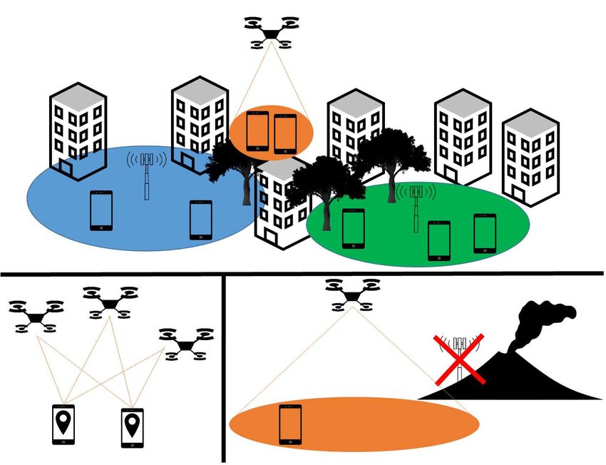
Fig. 1. Aerial User Equipment and Aerial Base Station scenarios
Fig. 2. Important performance metrics for different UAV-enabled wireless communication systems
The market size and dynamics resulted in a significant interest from the academia and industry in
UAV-based solutions. In this work, we give a comprehensive overview of the progress and challenges
that drone-enabled wireless communications face nowadays.
A. Aerial Wireless Communication
Drones can act as flying User Equipment (UE) (see Figure 1, left side). For instance, a UAV equipped
with a camera (and other necessary sensors) can provide a cost efficient solution for surveillance, in-
spection, and delivery. In this case, so-called Aerial User Equipment (AUE) has to co-exist with ground
users and exploit existing infrastructure (such as cellular networks) to transfer collected information to
the operator on the ground with certain reliability, throughput, and delay, depending on the application
requirements.
On the other hand, the use of a UAV-mounted Base Station (BS) is an alternative future technology
that can provide power-efficient wireless connectivity for ground users (see Figure 1, right side). Due to
its mobility and flexibility, an Aerial Base Station (ABS) can dynamically provide additional capacity
on-demand. This solution can be used by service providers both for dynamic network densification, fast
network deployment in an emergency situation, or temporary coverage of an area. Moreover, due to the
favorable propagation conditions the localization service precision can be significantly improved. Note
that the interference to the ground infrastructure also has to be taken into account.
UAV-enabled wireless communication networks have to be studied taking into account appropriate
channel models1 , antenna configurations, (A)UE and (A)BS densities, and other network parameters. A
coverage and reliability analysis is very different in both scenarios (see Figure 2).
1
Note that a complete channel model consists of Path Loss (PL), Large-Scale fading (LS-fading), and Small-Scale fading (SS-fading) models
considering the 3D location of both terminals, environment (rural, sub-urban, urban, etc.), frequency, and other physical link parameters.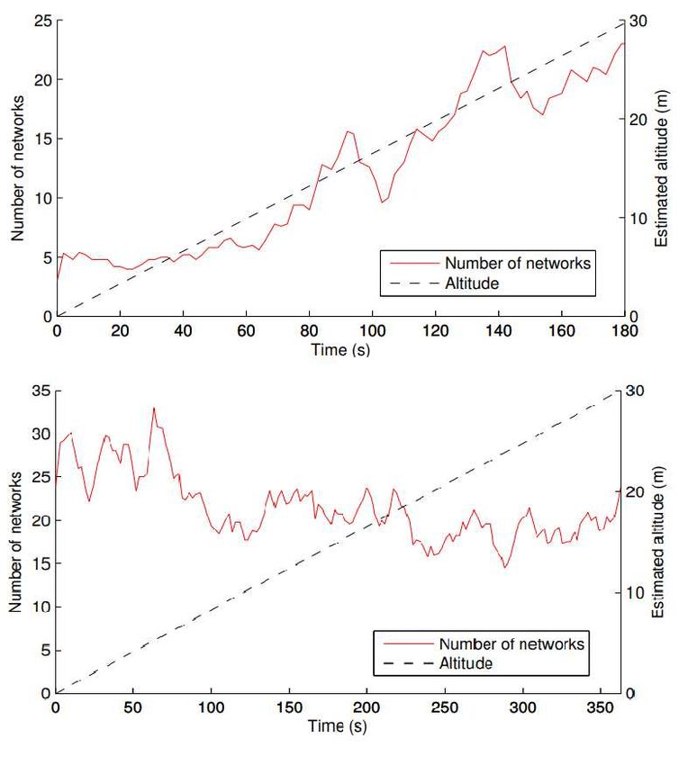
TUTORIAL ON UAVS: A BLUE SKY VIEW ON WIRELESS COMMUNICATION                                              3

                                                       TABLE I
                                                   UAV-related works

                                            PL: With            PL: Without       SS       Measurement
                                           LOS/NLOS             LOS/NLOS       -fading       -based
                                            separation           separation
                                        Fixed         3D           Fixed
                                        PLE         variant         PLE
                                                     PLE
                                      [14], [15]   [16], [17]    [18]–[21]    [16], [22]    [16], [22]
                                                   [22], [23]    [24], [25]   [18]–[21]     [18]–[21]
                   Channel modeling                [26], [27]                 [26], [28]    [26], [28]
                                                                              [24], [25]    [24], [25]
                                                                              [27], [29]    [27], [29]

                                        [30]       [31], [32]    [33], [34]   [30], [32]     [1], [35]
                        AUE                           [36]                    [31], [36]    [37], [38]
                                                                                            [33], [39]
                                                   [40], [41]    [42], [43]   [40], [42]
                        ABS                        [44], [45]    [37], [46]   [41], [44]
                                                                                              [43]
                                                   [47], [48]    [49], [50]   [37], [45]
                                                      [8]

   The first scenario requires a good link from the AUE to at least one of the BSs deployed, typically at
the rooftop level. At the same time, the other BSs become interferers and cause a performance drop. In
this scenario, the main focus is at the AUE performance, however, its coexistence with the terrestrial UEs
and the network infrastructure has to be studied.
   The second scenario requires a good link between all of the ground UEs to one of the multiple ABSs.
The radio wave propagation conditions are completely different for aerial channels when compared with
the terrestrial channels. Moreover, due to the aforementioned difference in the ground nodes (BS and
UE) height for the AUE and ABS scenarios, the propagation conditions significantly change. Another
important issue is that the aggregate interference to and from the air is different. Consequently, the
techniques and services designed for classical wireless networks (e.g. localization) have to be adapted to
the new 3D paradigm. It is obvious that completely different approaches are necessary for AUE and ABS
performance analysis.

B. Literature Review and Important Research Questions
   UAV communication performance analysis has attracted a large body of research so far. Papers focus
on the channel modeling only, or on system performance evaluation both for AUEs or ABSs. A detailed
overview of the published research is given in Table I. We can broadly classify the approaches: the
theoretical analysis (e.g. using the published channel models as a tool for AUE or ABS performance
estimation) versus measurement based research.
   The channel model should accurately reflect the environment seen by the wireless link to ensure a
correct and accurate performance analysis of the AUE and ABS communication. As it can be seen, the
main trend is to develop and use channel models differentiating two kinds of propagation: Line-of-Sight
(LOS) and Non-Line-of-Sight (NLOS). Moreover, the most elaborated of these models use an altitude-
dependent Path Loss Exponent (PLE). Several AUE and ABS performance analysis papers consider SS-
fading, which indeed makes those works more complete and realistic. Here we highlight main research
challenges, summarize the previously published literature, and discuss its limitations.
   1) Channel modeling: Channel modeling is one of the fundamental issues for designing any wireless
technology. Ground-to-ground networks are understood and modeled very well. In contrast, aerial commu-
nication channels have been investigated much less. The main challenge in Air-to-ground (A2G) channel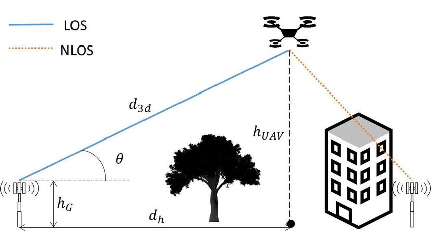
TUTORIAL ON UAVS: A BLUE SKY VIEW ON WIRELESS COMMUNICATION                                                4

modeling is the complexity of 3D environments and a large set of parameters that must be considered:
PL, LS-fading, and SS-fading behavior depends on the environment type (urban, rural, etc.), transmitter
(Tx) and receiver (Rx) heights, incident and/or elevation angles, the carrier frequency, LOS probability,
etc. Future techniques like millimeter wave (mmWave) and Massive-Multiple-In-Multiple-Out (MaMIMO)
still need to be studied in depth to improve their channel models in the aerial context.
   The aeronautical channel models survey in [19] discusses many channel modeling efforts, but these
models can only be used for aircrafts flying higher than the operating altitude of a typical commercial
drone. Several models of an aerial channel for lower heights have been proposed in literature (see Table I).
Well-known log-distance and two-ray PL models were parameterized via measurement campaigns. Some
works (e.g. in [22]) in fact, parameterized two separate models: for LOS and NLOS cases, whereas [18]–
[21] did not draw this distinction. In [23], an analytical model was presented. Measurement campaigns
suggest that SS-fading is usually Rayleigh or Nakagami distributed. Most of the time, published work
uses a statistical approach, whereas [51] proposes to use a Ray-tracing tool to model the channel.
   In this tutorial, we provide a comprehensive overview of existing channel models that can be directly
used for practical UAV applications as well as for research. We draw an explicit separation between
different propagation slices (or echelons): the ground level (below 10 m and 22.5 m for suburban and
urban environments, respectively), obstructed A2G channel (10 - 40 m and 22.5 - 100 m), and high-
altitude A2G channel (40 - 300 m and 100 - 300 m). Then we provide the model parameters for each
slice. Moreover, we show examples of the practical implementation of these models for simulation based
performance estimation of several drone-enabled scenarios.
   2) Aerial user equipment: AUE performance investigation is needed since the majority of wireless
technologies are not designed to operate in A2G links. Therefore, the performance is unpredictable in
such peculiar environments. Recent reports have concluded that interference is the main source of AUE
performance degradation Consequently, the main challenge is to estimate the performance taking into
account a complex propagation channel (see above) and the terrestrial network topology (BS density and
location, Tx power, 3D antenna patterns). Furthermore, coexistence of AUE with ground UE must be
investigated .
   Numerous research activities in this topic are well summarized in the surveys [6], [10], [36], [37],
[52], [53] where the requirements for quality-of-service, data, connectivity, adaptability, security etc.
were quantified. In [10], possible aerial network architectures were inspected, whereas [52] reports the
characteristics and requirements for UAV-networks for several promising civil applications. Some separate
use-cases were investigated in [6], [53]: it was underlined that for entertainment and virtual reality
applications, the communication channel can become the main limiting factor. AUE performance was
analyzed in [36] using a simulator consisting of PL channel model and 3D antenna patterns. Based on
measurements introduced in [37], it was concluded that the interference is one of the main problems
for AUE scenarios. The measurement-based performance estimation (see Table I) considers specific
environments and does not provide a unified framework for the AUE performance analysis. The results
presented in [30], [33], [34] use a channel model with a fixed PLE (independent of altitude), however,
only [30] considers the effect of SS-fading.
   While existing literature considers many important issues, it has some limitations. The surveys are
limited to isolated UAV application use-cases, so that the information is fragmented. A work that considers
all possible aspects and approaches to the AUE wireless communication performance estimation (from
theoretical analysis to experimental results) is missing, to the best of our knowledge. This knowledge is
the key to optimize future cellular networks while considering aerial usersnodes
   In this tutorial we give an overview of the theoretical state-of-the-art. We proceed with the simulation
based performance estimation of a cellular network serving an AUE. Next, we complete the study by giving
an overview of relevant measurement campaigns detailing the currently achieved UAV communication for
existing communication technologies such as LTE and Wi-Fi. We show that by considering the impacts
of the altitude, environments, antenna configuration, and network density, the UAV position potentially
can be optimized in order to achieve the highest coverage possibility.
TUTORIAL ON UAVS: A BLUE SKY VIEW ON WIRELESS COMMUNICATION                                               5

C. Aerial communication infrastructure
   ABSs, aerial relays on ad hoc networks, and are a promising addition to the conventional wireless
networks. It is vital to understand whether the use of ABSs is beneficial. Consequently, the main challenge
is to propose guidelines for the optimal 3D positioning, ABS deployment density, and path-planning (when
the UAV carrying the communication equipment is mobile) maximizing the advantages of ABS over the
conventional terrestrial BSs. The complete analysis should take into account the complex propagation
channel, antenna patterns, practical limitations (e.g. power consumption, weight or maximum flight alti-
tude) or required network performance metrics.
   Multiple papers listed in Table I consider mostly specific use cases and/or communication aspects
without providing a theoretical framework that could be used for a complete analysis of an aerial
communication network. Survey [43] investigates the optimal positioning of a helikite-mounted ABS
as well as considers more practical aspects such as dimensions and required power. The survey provides
measurement results, but the analytical results are limited: a very basic channel model is used and no
framework is proposed. An overview of ABS-aided networks is given in [9], however, it also lacks the
theoretical analysis and appropriate attention to the used channel models.
   In this work, we aim to provide a comprehensive overview on how UAV-mounted user equipment can
be used as a part of the communication network. Based on the theoretical analysis, we show how one
can optimize the coverage area of ABSs. The size of this area is a function of several parameters, e.g.
UAV height, transmit power and antenna tilt. The presented framework allows estimating the effect of
these parameters on the ABS system and optimal deployment configuration. Moreover, the influence of
multiple ABSs can be investigated. Similar to terrestrial BSs, multiple ABSs interfere with each other.
Therefore, the density of these ABSs must be studied to maximize the coverage of the network, while
minimizing the interference. Additionally, the parameters important for ABS’s deployment is studied to
optimize the localization service they will provide. For example, we analyze how the height of the UAV
influences the positioning error of the localization system.

D. Tutorial Organization
   Summarizing, the main contributions of this article is the overview and tutorial on the wireless com-
munications for UAV. Our purpose is to provide an introduction of the UAV wireless communications to
the reader not working in this topic but interested in getting a general introduction to the subject. This
tutorial also targets researchers wishing to get a comprehensive background before working on the subject.
The main goal is to gather and systematize the vast, but fragmented state-of-the-art research contributions
regarding most important aspects of UAV-enabled wireless communications networks.
   The tutorial is structured as follows:
   • Section II provides an overview of the motivating UAV applications for both scenarios: UAV as the
     UE or UAV as integral part of the communication system.
   • Section III is focused on the UAV communication basics, mainly giving an overview of the main
     Air-to-air (A2A) and A2G channel models taking into account PL, LS-fading, and SS-fading. These
     models consider the 3D location of both terminals, environment, frequency, and other important
     physical link parameters. The guidelines on how the models can be applied are given.
   • Section IV discusses the communication performance for UAVs as an AUE scenarios, focusing on
     analytical, simulation, and measurement results.
   • Section V discusses two promising UAV applications when they are a part of the network infras-
     tructure. First, we present an analytical communication performance estimation for ABSs followed
     by performance simulations. Next, we discuss the localization performance, for scenarios where the
     UAV is a part of a localization system.
   • Section VI provides an overview of the future research directions and challenges.
   • Section VII concludes the paper.
TUTORIAL ON UAVS: A BLUE SKY VIEW ON WIRELESS COMMUNICATION 6
Fig. 3. Qualitative requirements for various use-cases when UAV acts as an UE
II. Wireless Communication for UAVs: Use Cases
A wide range of use cases can be imagined for UAVs. When analyzing the performance of UAV
communication, it is important to divide the use cases in two classes of scenarios, one where the UAV
is used as a mobile terminal and the second one where the UAV is a part of the wireless communication
infrastructure. In the first case, the UAV is considered as an AUE, where the data generated by the payload
of the UAV needs to be transmitted to serve an application. In the second case, the UAV is exploited
as a part of the communication system, for example, as a mobile base station or anchor for localization
of Internet of Things (IoT) devices. Below, we first describe some scenarios where the UAV is a mobile
wireless terminal, and then we focus on scenarios where the UAV is part of the infrastructure.
A. Unmanned Aerial Vehicles as User Equipment
Naturally, drones can act as users of the wireless infrastructure. To properly use drones as AUE, the
requirements for the communication between drones and ground infrastructure should be adapted to the
considered application (see Figure 3). For instance, it is obvious that for search and rescue, the reliability
is vital. In the case when the UAV-mounted camera is used to help a ground-based operational center,
the delay and throughput requirements are high. However, due to the possibility of augmenting the UAV
with autonomous on-board functionality such as positioning and person detection, the drone can also only
transmit the coordinates of the person.
Many studies are dedicated to the feasibility of AUE usage in existing cellular networks (see Table I).
It turns out that the interference becomes the main limiting factor for the wide deployment of the cellular-
connected drones due to the fact that current cellular networks were designed for ground users whose
operations, mobility, and traffic characteristics are substantially different from the AUE.
There are key differences between drone-mounted and ground UEs. The propagation conditions for
A2G and terrestrial channels are completely different due to nearly LOS communications between ground
BSs and AUEs. On one hand, it improves the received signal level, but in return the interference from
the other BSs also grows. Moreover, the ground users are in general less dynamic than UAVs, therefore,
the techniques used currently in the cellular networks might require significant modification to enable the
highly mobile users.
In the case of an AUE, it may need to transfer the information about to the security operation center. This
information might vary from telemetry-like signals to a more demanding video stream. Let us describe
the most promising AUE applications.
1) Search and Rescue: Drones have been used for searching victims [4]. Due to the freedom of mobility,
they can be used in various dangerous scenarios. The authors of [54] proposed a specialized UAV platform
to search and rescue people in case of avalanches, which is capable of locating survivors fast, and hence
ensuring a maximal survival chance. Furthermore, when fitted with the right sensors, UAVs can also be
used for indoor and outdoor urban rescue missions [55]. As a results, from May 2017 through April 2018,
DJI has counted 65 people who were rescued from peril by use of a drone [56]. Recently, drones alsoTUTORIAL ON UAVS: A BLUE SKY VIEW ON WIRELESS COMMUNICATION 7 proved to be a perfect tool to prevent casualties. The Los Angeles Times reported [57], that infrared drone footage, taken from high altitude, informed a group of firefighters near Yosemite National Park, that they were facing seven spot fires instead of just one they had been aware of. Moreover, after a fire burned, drones are ideal for damage assessment as it has been done after wild fires in Greece [58]. 2) Security: UAVs are able to optimize their path quickly and complete complex missions due to their high mobility, which makes them attractive for various security and safety-related applications. Equipped with the right sensors and actuators, UAVs can monitor an area for illegal activities via video surveillance. For surveillance purposes, [59] describes a method to detect humans on aerial footage and estimate the pose and trajectory of the subjects. In addition, multiple drones can be controlled by one ground control station to dynamically secure a large area [60]. Other UAVs can be used in order to detect [61] and/or intercept [62] malicious drones, e.g. drones equipped with a net can catch malicious UAVs. 3) Entertainment and Media: The entertainment business was one of the first businesses to widely use drones for the production of TV shows and movies. But for these applications, the video is stored on board on the UAV. In the future, there are plans to use drones for live broadcasting and AR/VR applications [53], this requires a reliable high-throughput link to safely transmit the stream from the drone to the ground operating center. Another option is to use drones as broadcasting relays. For big sports events, like bikes races, motorcy- cles are used to film the athletes. The stream gets relayed via a helicopter to the control station of the TV station. Operating this helicopter is not cost efficient, therefore an UAV could be equipped with relaying infrastructure [63] and autonomously optimize its position to retransmit the video streams. Another example of an entertainment application for drones comes from Intel, which uses drones to make animated light shows [64]. These Intel Shooting Star drones are fitted with LED bulbs and fly in formation to form breath taking displays. In order to coordinate the movement from more than a thousand drones, a reliable and low-latency communication system is needed that sends the correct commands to all the drones. The next application for entertainment purposes came from Dolce & Gabbana. During their Winter 2018 showcase in Milan, they demonstrated their handbags and purses by flying them down the catwalk using drones [65]. 4) Inspection: Autonomous UAV can easily take over when highly repetitive flights (such as a periodic industrial infrastructure inspection) have to be performed. An example is the inspection of wind turbine blades for damage and wear. When checking the blades of an entire wind turbine park, the pilot can loose the concentration. This leads to dangerous situations where the pilot could crash or miss a damaged spot on the turbines blades. Autonomous drones rely on cameras and software to do these routine inspections and do not have the problem of fatigue, therefore the inspections will become more secure and effective. The same procedure can also be applied on other big industrial installations e.g. petrochemical plants and cooling towers [66]. Several projects and companies are already dedicated to this use case, like SkySpecs [67] and SafeDroneWare [5], [68]. 5) Traffic Monitoring: Owing to their dynamic and multidisciplinary characteristics, drones have be- come increasingly popular for traffic monitoring. This interest resulted in several research activities. One of the first related surveys [6] concludes that UAVs are proven to be a viable and less time-consuming alternative to real-time traffic monitoring and management, providing the eye-in-the-sky solution to the problem. The main functions that an aerial-based traffic monitoring system should have are i) object (pedestrian, car etc.) detection [69], [70], ii) tracking [71] and iii) analysis of the collected information (e.g. the flow density and dynamics) [72]. In addition, UAVs can be deployed on demand in a fast and dynamic way. This can be extremely interesting for sudden traffic jams due to accidents or large events. The monitoring services at these locations will help to avoid traffic jams at these locations in the future.
TUTORIAL ON UAVS: A BLUE SKY VIEW ON WIRELESS COMMUNICATION                                                                         8

Fig. 4. Aerial Base Station use cases. Top: Future communication networks; Bottom, Left: Localization service; Bottom, Right: disaster
scenario

B. Unmanned Aerial Infrastructure
   1) Aerial Base Stations: Future Telecommunication Networks: The demand for high-speed wireless
access has been incessantly growing last years. Smart-phone traffic will exceed PC traffic by 2021: traffic
from wireless and mobile devices will account for more than 63 percent of total IP traffic by 2021 [73].
The interest in enhancing the capacity and coverage of existing wireless cellular networks has led to
the emergence of new wireless technologies, which include ultra-dense small cell networks, mmWave
communications and MaMIMO. They often are collectively referred as the next-generation 5G cellular
systems.
   We believe that UAV-mounted base stations will become an important component of the 5G environment
due to the ability of providing on-demand connectivity to the users at little additional cost [48] as shown
in Figure 4 (top). Meanwhile, a mmWave ABS mounted on a UAV [74] can naturally establish LOS
connections (which is vital for the wireless links at these frequencies) to ground users. In its turn,
combining mmWave communications and MaMIMO can be an attractive solution to provide high capacity
wireless transmissions.
   2) Aerial Base Stations: Public Safety During Natural Disasters: Natural disasters such as earthquakes,
fires, and floods often yield to severe damage or complete destruction of the existing terrestrial commu-
nication networks. In particular, cellular base stations and ground communication infrastructure is often
damaged and overloaded during natural disasters (see Figure 4, bottom right). It is obvious that there is a
need for public safety communication solutions for search and rescue operations. The potential broadband
wireless technologies for public safety scenarios include 4G Long Term Evolution (LTE), Wi-Fi, satellite
communications and dedicated public safety systems [11].
   An ABS can be seen as a part of a robust, fast, and capable emergency communication system enabling
effective communications during public safety operations[45]. For instance, AT&T deployed an LTE cell
site on a helicopter to connect residents after a disaster in Puerto Rico in 2017 [75]. However helicopters
have a high operating cost. While UAVs can easily fly and dynamically change their positions to ensure
TUTORIAL ON UAVS: A BLUE SKY VIEW ON WIRELESS COMMUNICATION                                                                          9

full coverage to a given area within a minimum possible time and at a low operating cost. Therefore, the
UAV-mounted base stations can be seen as the key enabler for providing fast and ubiquitous connectivity
in public safety scenarios.
   3) Aerial Anchors: Positioning for Ground Users: Another advantage of using drones as part of the
wireless infrastructure, is that they can be used for localization of terrestrial nodes (see Figure 4, bottom
left). Aerial positioning systems have the advantage of having a higher LOS-probability than a terrestrial
BS, which increases the possible positioning-accuracy. [76] envisions a localization system based on
aerial anchors, where terrestrial users can localize themselves using the Received Signal Strength (RSS)
of three or more static UAVs. [77] proves that these drones can also be replaced by one single drone
if the users are static. Other proposed systems make use of time-based approach. Both of them have
advantages and disadvantages. RSS based systems can use already available data to calculate the position
of the device hence, this strategy is very power efficient. This comes with the drawback of being less
accurate. Therefore, this option is ideal for static battery powered IoT devices, since their main limitation
is battery-stored energy. Moreover, since these devices are not mobile, the accuracy error can be lowered
by averaging over time. These characteristics make this system a viable option over Global Positioning
System (GPS) to position static IoT devices. Time-based systems can be used to complement GPS signals
to further enhance the positioning accuracy. This is possible due to their higher accuracy than the RSS-
based systems. However, they do need a very accurate clock signal at the transmitter and the receiver,
which requires a substantial amount of energy to operate. Both technologies can have potential to enhance
the current available positioning and to achieve higher energy efficiency or higher accuracy.

                                  III. Fundamentals of UAV Communication
   In wireless communication networks, the propagation channel is the medium between the transmitter
and the receiver. It is obvious that its properties influence the performance of wireless networks. Next gen-
eration UAV-enabled networks design (i.e., algorithms development) is impossible without the knowledge
of the wireless channel. Consequently, radio channel characterization and modeling in such innovative
architectures becomes crucial to evaluate the achievable network performance.
   The vast majority of the channel modeling efforts is dedicated to terrestrial radio channels. Unfortunately,
wireless communication with UAVs cannot rely on these models. The nature of A2G channels implies
a higher probability of LOS propagation. This results in a higher link reliability and lower transmission
power. Even for NLOS links, power variations are less severe than in the terrestrial communication
networks due to the fact that only the ground-based side of the link is surrounded by the objects that
affect the propagation. Figure 5 illustrates A2G propagation channel and introduces the main geometrical
parameters as well as drawing the important distinction between LOS and NLOS channels2 . On the other
hand, the UAV mobility causes high rates of change. Modeling of these changes is challenging due
to arbitrary mobility patterns and complex operational environment. Doppler shift caused by the UAV
motions has to be taken into account as well.
   Apart from the channel itself, there are other factors that influence the received power strength such
as: airframe shadowing, self-interference from the on-board devices and antenna characteristics.
   An accurate channel model of A2G channels is vital for design and optimal deployment of the
communication networks including UAVs as its nodes. In this section we will discuss a number of research
questions and recent efforts dedicated to this important issue.

A. Background
  The transmitter radiates electromagnetic waves in several directions. Waves interact with the surrounding
environment through various propagation phenomena before they reach the receiver. As illustrated in
  2
    There is no trivial dependency between any of these parameters and the performance metrics described in the following sections. Any
change of the link geometry results in a complex change of the network operation.
TUTORIAL ON UAVS: A BLUE SKY VIEW ON WIRELESS COMMUNICATION 10
Fig. 5. Air-to-Ground propagation
Fig. 6. Air-to-ground propagation
Figure 6, different phenomena such as specular reflections, diffraction, scattering, penetration or any com-
bination of these can be involved in propagation [78]. Therefore, multiple realizations of the transmitted
signal, often termed as Multi-path component (MPC) arrive to the Rx with different amplitudes, delays
and directions. The resulting signal is the linear coherent superposition of all copies of the transmitted
signal, which can be constructive or destructive depending upon their respective random phases.
Typically, radio channels can be represented as a superposition of several separate fading mechanisms:
H = Λ + XLS + XS S , (1)
where, Λ is the distance dependent PL, XLS is the LS-fading (also known as shadowing) consisting of
large scale power variations caused by the environment, and XS S is the SS-fading (see Figure 7).
Depending on the altitude, different channel models (or their parameters such as PLE or LOS probability)
must be used due to the obvious difference in experienced propagation conditions. The airspace is often
separated into three propagation slices (or echelons):
• Ground level: below 10 m or 22.5 m for suburban and urban environments, respectively [16]. These
channels can be modeled by using terrestrial channel models since the aerial node altitude is below
the rooftop level. Mostly the NLOS propagation is expected.
• Obstructed A2G channel: 10 - 40 m and 22.5 - 100 m for suburban and urban environments,
respectively. These channels experience a higher LOS probability than the ground channels, however,
it is not 100%. Consequently, a large variation of the received power around the mean Signal-to-
Noise-Ratio (SNR) levels is observed.TUTORIAL ON UAVS: A BLUE SKY VIEW ON WIRELESS COMMUNICATION 11
-40
Small-scale fading
Pathloss
-60 Large-scale fading
Channel, [dB]
-80
-100
-120
-140
0 500 1000 1500 2000
Distance, m
Fig. 7. Channel components
High-altitude A2G channel: 40 - 300 m and 100 - 300 m. Above certain altitude (depending on the
•
environment), all channels are in LOS, so the propagation is close to the free-space case. Consequently,
only LOS channel model can be used. Moreover, no LS-fading is expected.
Additionally, A2A channels are mostly experiencing LOS propagation and similar to the high-altitude
A2G channels. Note that in this case, the UAVs mobility can be significantly higher which causes larger
Doppler shifts.
Next, let us describe models of the components presented in (1) separately.
1) Path Loss and Large-Scale Fading:
a) Air-to-Air channels:: The simplest path-loss model assumes a LOS link between the Tx and Rx
and propagation in free space. This assumption represents well the situation when two UAVs communi-
cating with each other (so-called A2A channels) at a relatively high altitude (above the rooftop level). In
this case, the received signal power is given as [79]
!2
λ
PR = PT G T G R , (2)
4πd
where PT is the transmitted power, GT and GR are the transmit and receive antenna gains, respectively, λ
is the carrier wavelength, and d is the distance between the Tx and Rx3 . Note that the PLE η (the power
of the distance dependence) in this equation is 2 for free-space propagation. So that the path loss can be
expressed for a generalized case as !η
4πd
Λ= . (3)
λ
b) Air-to-Ground channels:: Unfortunately, the signals in real-life A2G wireless communications
do not experience free space propagation. In the majority of literature, the well-known log-distance PL
model with free-space propagation reference is used for PL (in dB) modeling:
Λ(d) = Λ0 + 10η log(d/d0 ), (4)
h 4πd i
where Λ0 is the PL at reference distance d0 (Λ0 can be specified or calculated as free space PL 20 log λ 0 ).
When the deterministic path-loss is removed, mean power, averaged over about 10-40 wavelengths,
itself shows fluctuations over time. These random variations of locally averaged received power over
large distances, typically on the order of a few tens or hundreds wavelengths, are known as LS-fading,
3
For simplicity of notation, d = d3d in Figure 5TUTORIAL ON UAVS: A BLUE SKY VIEW ON WIRELESS COMMUNICATION 12
due to large obstacles such as buildings, vegetation, vehicles, the UAV’s airframe etc. The obstacles
affecting the propagation of radio signal can be very different from each other, resulting in large-scale
variations at different locations, while having approximately the same Tx-Rx distance. At any distance d,
LS fading XLS measured in dB is usually modeled as a normal random variable with a variance σ, which
takes into account random variations of the received power around the path loss curve. This model is
attractive since it is widely used (with different parameters) for modeling of classical terrestrial channels.
Another common PL model used in the literature [7], [8], [16], [23], [40], [44], separates the path loss
into two components namely LOS and NLOS:
Λavg = PLOS · ΛLOS + (1 − PLOS ) · ΛNLOS , (5)
where ΛLOS ,NLOS are the path loss for the LOS and NLOS cases, respectively, PLOS denotes the probability
of having a LOS link between the UAV and the ground node. An advantage of this model is that PLOS
calculation can be adapted to different heights of the communicating terminals so that we can take into
account the difference between the scenarios when the aerial node communicates with a node located at
low altitudes (≤ 2 m) or with a BS, which typically are deployed higher.
2) Small-Scale Fading: Small-scale fading describes the random fluctuations of the received power
over short distances, typically a few wavelengths, due to constructive or destructive interference of MPCs
impinging at the receiver. Different distributions are proposed to characterize the random fading behavior of
the signal envelope, suitable for different wireless systems and propagation environments. The Rayleigh
and Rice distributions, both based on a complex Gaussian distribution, are the most commonly used
models. Considering a large number of MPCs with amplitudes and random phases, the signal envelope
of small-scale fading thus follows a Rayleigh distribution [79]. For A2A and A2G channels, where the
impact of LOS propagation is high, the Ricean distribution [79] provides a better fit.
Small-scale fading models apply to narrow-band channels or taps in tapped delay line wideband models.
Due to the stochastic nature of these signal variations, fading is usually modeled using statistical approaches
and its models are obtained through measurements or through geometric analysis and simulations. The
most popular type of small-scale models is Geometry-Based Stochastic Channel Models (GBSCM) [78].
B. Important Results
Now, let us present the parameters of the most popular models so that one can choose the appropriate
modeling approach.
1) Path Loss and Large-Scale Fading Modeling:
a) Log-distance models:: In Table II, the parameters of the PL log-distance model presented in
(4) as well as the standard deviation for the Normal distribution N(0, σ2 ) describing LS-fading can be
found. Note that these results are valid for the frequency ranges and environments considered for the
measurement campaigns used to parameterize the model. For mmWave, atmospheric absorption and rain
attenuation can also lead to a significant power loss. For example, at 28 GHz, the attenuations caused
by atmospheric absorption and heavy rain over a distance of 200 m are about 0.012 dB and 1.4 dB as
reported in [83].
In the case when the distinction between LOS and NLOS situations is made (i.e. when (5) is used),
the critical point is the LOS probability PLOS modeling. In [23], it is given by
Y m h
[hU AV − (n+1/2)(h
m+1
UAV −hG ) 2 i
]
PLOS = 1 − exp − 2
, (6)
n=0
2Ω
√
where we have m = f loor(dh ςξ−1) , dh is the horizontal distance between the UAV and the ground node,
hU AV and hG are the terminal heights, ς is the ratio of land area covered by buildings compared to the total
land area, ξ is the mean number of buildings per km2 , and Ω is the scale parameter of building heights
distribution (assumed to follow Rayleigh distribution [84]). In some cases, it is more convenient to express
the LOS probability as a function of incident or elevation angle (e.g. in [41]). These representations can
be found in [17], [41].TUTORIAL ON UAVS: A BLUE SKY VIEW ON WIRELESS COMMUNICATION 13
TABLE II
Parameters of Pathloss and Large-scale fading models
Scenario Frequency, GHz η Λ0 , dB σ, dB Reference
2.54-3.037 21.9-34.9 2.79-5.3 [22]
2.2-2.6 [14]
2.01 [15]
Suburban, 4.1 5.24 [80]
Urban, Open 2-2.25 [27]
field 0.968 1.6 102.3 [21]
5.06 1.9 113.9 [21]
0.968 1.7 98.2-99.4 2.6-3.1 [18]
5.06 1.5-2 110.4-116.7 2.9-3.2 [18]
Over sea 1.4-2.46 19-129 [81]
Mountains 1-1.8 96.1-123.9 2.2-3.9 [24]
Urban (LOS) 28 2.1 3.6
Urban (NLOS) 28 3.4 9.7
Urban (LOS) 38 1.9-2 1.8-4.4
[82]
Urban (NLOS) 38 2.2-2.8 4.1-10.8
Urban (LOS) 73 2 4.2-5.2
Urban (NLOS) 73 3.3-3.5 7.6-7.9
TABLE III
Large-scale fading model parameters
σ, dB Applicability
4 LOS, Ground level, 10 m ≤ dh ≤ d2
6 LOS, Ground level, d2 m ≤ dh ≤ 10 km
8 NLOS, Ground level
4.2 exp(−0.00046hUAV ) LOS, Obstructed LOS and High-altitude A2G
6 NLOS, Obstructed LOS A2G
b) Ground level channel models:: When the airspace is divided into slices, the channel is modeled in
different ways depending on the UAV altitude. The ground level (1.5 m < hU AV ≤ 10) is the one providing
the richest choice of possible channel models since the well-known models designed for conventional
cellular networks can be used. In this tutorial, let us describe just one of the options provided by 3rd
Generation Partnership Project (3GPP) for macro-cell networks deployed in rural environments4 in [16],
[85].
Again, since the LOS and NLOS cases are treated separately, the LOS probability has to be calculated.
It is expressed as
1 if dh ≤ 10 m
(
PLOS = dh −10 (7)
exp − 1000 if 10 m < dh
As soon as the LOS probability is known, the PL and LS-fading can be calculated. The altitude dependent
LS-fading can be modeled as N(0, σ2) with the parameters listed in Table III.
It has been pointed out that the PL changes with the position of the communication nodes and can be
calculated as: (
G Λ1 if 10 m ≤ dh ≤ d2
ΛLOS = , (8)
Λ2 if d2 ≤ dh ≤ 10 km
ΛGNLOS = max(ΛGLOS , Λ′NLOS ) for 10 m ≤ dh ≤ 5 km , (9)
4
expressions for other environments and micro-cell deployment can be found in [16], [85]TUTORIAL ON UAVS: A BLUE SKY VIEW ON WIRELESS COMMUNICATION 14
where
Λ1 = 20 log(40πd3d fc /3) + min(0.03h1.72 1.72
U AV , 10) · log d3d − min(0.044hU AV , 14.77) + 0.002d3d log hU AV ,
d3d
Λ2 = Λ1 + 40 log ,
d2
Λ′NLOS =161.04 − 7.1 log W + 7.5 log hU AV − (24.37 − 3.7(hU AV /hG )2 ) · log hG +
+ (43.42 − 3.1 log hG )(log d3d − 3) + 20 log fc − (3.2 log(11.75hU AV ))2 − 4.97),
d2 = 2πhU AV hG fc /c.
In the expressions above fc , hB , W, c are the carrier frequency, average building height, the average street
width, and the speed of light, respectively.
c) Obstructed air-to-ground channel models:: The next air-space slice considers the UAV altitudes
10 m < hU AV ≤ 40 m, where the LOS probability in macro-cell networks in rural environments is calculated
as in [16]:
1 if dh ≤ d1 ,
(
PLOS = d1 −d −d1 (10)
dh
+ exp p1 1 − dh
h
if d1 < dh
where
p1 = max(15021 log(hU AV ) − 16053, 1000),
d1 = max(1350.8 log(hU AV ) − 1602, 18).
Next, the PL for LOS and NLOS cases can be calculated as
40π fc
ΛALOS = max(23.9 − 1.8 log hU AV , 20) log d3d + 20 log , (11)
3
40π fc
ΛANLOS = max(ΛALOS , −12 + (35 − 5.3 log hU AV ) log d3d + 20 log . (12)
3
d) High-altitude air-to-ground channel models:: For the 40 m < hU AV ≤ 300 m, the LOS probability
equals 1 and PL can be calculated as in (11).
2) Small-Scale Fading Modeling: As previously noted, the most common small scale fading distribution
for A2G propagation is the Ricean [40]. In general, A2G channels expose a higher influence of LOS-
components than an average terrestrial link. As in terrestrial channels, for the NLOS case, the Rayleigh
fading distribution typically provides a better fit [27], [80] and of course, other distributions such as the
Nakagami[30], chi-squared (χ2 ) and non-central χ2 [42], [44], and Weibull distributions might also be
employed. The family of χ2 distributions is attracting our attention since many of the distributions listed
above are particular cases of it.
In [16], several algorithms of generating small-scale fading are provided. One of these alternatives
suggests that the small-scale model is used with a K-factor of 15 dB and all the remaining parameters are
reused from the well-known terrestrial model in [85], including the delay and angular spreads, the cross-
correlations among the large-scale parameters, the delay scaling factor, the number of clusters, the cluster
delay and angular spreads, etc. This is the simplest of the suggested algorithms, the other alternative can
be found in [16].
Note that the PL, LS-fading and SS-fading models and their parameters for urban and micro-cell
scenarios can be found in [16], [85].TUTORIAL ON UAVS: A BLUE SKY VIEW ON WIRELESS COMMUNICATION 15
3) Conclusions: The choice of an adequate channel model depends on the targeted result. When an
approximate result is needed for a large set of areas, it is practical to apply a simple channel model that
will reproduce the general propagation trends. For instance, the log-distance model with a fixed PLE is an
appropriate choice. However, in the case when a more specific environment is to be investigated, a more
complex channel model might be necessary. The most complete air-to-ground channel models consider:
• Path loss, large- and small-scale fading mechanisms,
• Propagation slice (ground, obstructed A2G, high-altitude A2G),
• Different environment types (urban, suburban, rural, open),
• Separate parameterization of LOS and NLOS models.
In this section we presented the whole spectrum of statistical channel models that can be applied depending
on the final goal.
IV. Aerial User Equipment Communication Performance
In this Section, we detail the state-of-the-art results in the communication performance analysis for
UAV networks, in scenarios where the UAV is considered to be a UE or mobile terminal. We start with
an overview of the theoretical state-of-the-art, mainly concentrating on the the analytical works using
the channel models described in Section II, or more precisely we develop our performance analysis
framework based on the channel model separating LOS and NLOS propagation cases. Next, we present
the performance estimation of an LTE cellular network serving an UAV based on a simulator consisting
of a realistic 3-dimensional urban environment combined with semi-deterministic channel models. We
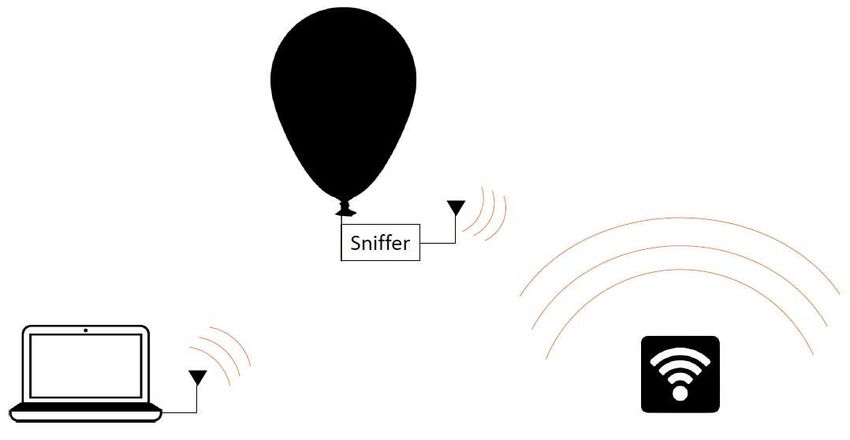
proceed by giving an overview of all relevant measurement campaigns detailing the currently achieved
UAV communication for existing communication technologies such as LTE and Wi-Fi.
A. Theoretical Performance Analysis
The feasibility of LTE-based UAV communication is often examined via field trials and simulations.
Such a focus on the experimental studies results in a highly fragmented picture of the issues related to the
cellular-based communication with drones. Surprisingly, the analytical investigation of AUE scenarios is
not widely studied in literature. We believe that the theoretical frameworks to analyze the coexistence of the
aerial and ground users [30] and the coverage probability [31] are necessary. In [32], we presented a generic
model to analyze the performance of UAVs served by a conventional cellular network. In this tutorial, for
simplicity reasons, we provide the results only for some specific cases that can be interesting from the
practical deployment point of view. Following characteristics are considered: i) coverage probability, ii)
achievable channel capacity, and iii) area spectral efficiency.
Here we aim to address theoretically the following important questions:
• are the current and future cellular networks capable of providing adequate quality of service for
AUEs?
• what are the major factors that may limit the network performance for AUEs?
• how does the flexibility of UAV design help to achieve better performance?
1) Network Architecture:
a) System architecture:: We consider a cellular network consisted of ground BSs, UE, and AUE.
A homogeneous Poisson point process (HPPP) Φ with density λ BSs/Km2 was used to model to BSs
locations. The BSs’ heights are denoted as hG as in (6).
Users are assumed to be located hU AV meters above the ground (note that for ground users h =1.5 m).
The horizontal distance dh separates a BS and a specific UE’s projection on the ground 0 (see Figure 8).
The BS antenna radiation pattern is imitating a realistic deployment (the antennas are vertically directional
and horizontally omnidirectional). The network is assumed to be optimized for the terrestrial users so that
the antennas are tilted down [86]. Consequently, the AUE is assumed to receive signals from the sidelobes.
The antenna gain of a BS is represented by G BS , with G M and Gm being the main- and side-lobe gains,
respectively.TUTORIAL ON UAVS: A BLUE SKY VIEW ON WIRELESS COMMUNICATION 16
Fig. 8. Network geometry
We consider that AUE is able to control the antenna tilt (mechanically or electrically). The AUE antenna
is characterized by its opening angle φB and tilt angle φt , as illustrated in Figure 8. We assume that the
UAV antenna gain is GU E = 29000/φ2B within the main lobe and zero outside of the main lobe [87]. As a
result, an AUE receives with sufficient gain only signals from BSs within an elliptical section, denoted by
C (see Figure 8). The communication link length d3d between a BS and a UE is defined as in Section II.
b) Channel model:: The approach presented in Section II, equation (5) is used so that the LOS
and NLOS components are treated separately with the probability of LOS modeled as in (6). Note that
the LOS probability of different communication links are assumed to be independent. When the LOS
probability is known, path loss is calculated as in (4) with the reference loss ΛL,N and PLE ηL,N for LOS
and NLOS links, respectively.
For modeling of the small-scale fading XS S ,υ (υ is chosen depending if the link is LOS or NLOS) we
use the Nakagami-m distribution, which contains a wide range of fading types as specific cases [88].
Accordingly, XS S ,υ follows a distribution with the cumulative distribution function (CDF)
m υ −1
X (mυ ω)k
F XS S ,υ (ω) , P[XS S ,υ < ω] = 1 − exp(−mυ ω), (13)
k=0
k!
where mυ is the fading parameter assumed to be a positive integer for the sake of analytical tractability.
Note that the larger mυ corresponds to lighter fading.
If a BS transmits with a power level PT x , the corresponding received power is given by
PRx (d3d ) = PT x G Λυ (d3d ) XS S ,υ , (14)
where G = G BS GU E represents the cumulative effect of transmitter and receiver antenna gains.
c) Performance metrics:: The system performance is estimated using three metrics derived from
Signal-to-Interference-and-Noise-Ratio (SINR) expressed as
PT x G Λυ (dh ) XS S ,υ
S INR = ; υ ∈ {L, N}. (15)
I + N0
The performance is affected by many system parameters including the AUE altitude, hU AV . Therefore,
all the metrics are dependent on these parameters, even if it is not expressed explicitly.
Coverage Probability denoted by Pcov reflects the reliability of the link between a UE and its associated
BS in satisfying the target requirement and it is defined as
Pcov , P[S INR > T], (16)
which can be written as Pcov = Pcov (hU AV , T) as SINR depends on hU AV . The target value T is determined
based on the user requirement and is related to the target rate RT x by T = 2RT x/BW − 1, where BW isTUTORIAL ON UAVS: A BLUE SKY VIEW ON WIRELESS COMMUNICATION 17
the bandwidth allocated to each user. Additionally, this metric is useful to evaluate the reliability of a
command and control link.
Channel Capacity denoted by R is the highest bit rate achievable by a UE in the network. This metric
can be calculated as
R , E log2 (1 + S INR) (b/s/Hz), (17)
which is the user altitude hU AV and the BS density λ dependent, and hence can be written as R = R(hU AV , λ).
While the coverage is useful to characterize the quality of service and reliability, the throughput R
quantifies performance in terms of average raw throughput. In other words, R and Pcov are complementary
for the BS to UE link quality estimation.
Area Spectral Efficiency (ASE) denoted by A, is a network-level performance metric that reflects the
achievable data-rate per square meter. Let us denote the ratio of UE to AUE numbers as ρ . In a given
area, the densities of BSs serving AUEs and ground users are λρ and λ(1 − ρ), respectively. Therefore,
the average throughput per square meter can be calculated as
A , λ[(1 − ρ) · R(1.5, λ) + ρ · R(hU AV , λ)] (b/s/Hz/Km2 ), (18)
where R(1.5, λ) and R(hU AV , λ) corresponds to ground users at altitude of 1.5 m and aerial users at altitude
of hU AV , respectively. This metric provides an insight into the overall effect of adding aerial users in the
network and how the overall spectrum efficiency changes when network resources are shared between
ground and aerial users.
2) Important Results:
a) Performance analysis:: Below, we present several results for the performance metrics described
above. Note that this tutorial contains only the expressions for the most popular practical cases (i.e.
omnidirectional AUE antenna is considered), for more generalized results refer to [32].
Coverage Probability - First, we present the expression for the downlink coverage probability of a
cellular-connected UAV equipped with an omnidirectional antenna in the case when the AUE is flying
higher than the serving BS. Given the system model and performance metrics defined earlier, it is obtained
as
Z re +r M
′
Pcov ≈ 2 Pcov | dh (d ) f (d′ )[π + ϕ1 (d′ ) − ϕ2 (d′ )] d′ dd ′ ,
0
L
where f (d ′) ≈ λP(d ′ ) · e−2λI1L is the probability density function (PDF) of the serving BS’s distance dh at
an arbitrary angular coordinate within C,
m L −1
X (−yL )k d k −2λIL
Pcov | dh ≈ · ke 2L , (19)
k=0
k! dy L
mL T
yL = ,
PT xGΛ(dh )
Z ∞ " !mL #
′ ′ mL
L
,
I2L d P(d )π 1 − dd ′
dh m L + y P
L Tx GΛ(d h )
Channel capacity and ASE - The achievable throughput of a typical UE can be obtained as
1
Z ∞
Pcov (hU AV , t)
K
1 X Pcov (hU AV , tn) π2 sin 2n−1
2K
π
R , E log2 (1 + S INR) = dt ≈ · h i,
ln 2 0 1+t ln 2 n=1 1 + tn 4K cos2 π4 cos 2n−1 π + π
2K 4
(20)
where the last equation is an approximation to facilitate numerical calculations. Note that parameter K
has to be chosen large enough for a high accuracy of the approximation [89]. Also, tn stands for
" ! #
π 2n − 1 π
tn = tan cos π + . (21)
4 2K 4
Finally, ASE is obtained by a direct substitution of R(hU AV , λ) from (20) into (18).TUTORIAL ON UAVS: A BLUE SKY VIEW ON WIRELESS COMMUNICATION 18
5
4
Throughput [b/s/Hz]
3
2
1
0
0 10 20 30 40 50 60 70 80 90 100
Altitude of UE [m]
Fig. 9. The impact of UAV altitude and environment on the performance of network.
7
6
Throughput [b/s/Hz]
5
4
3
2
1
0
100 110 120 130 140 150 160 170
UAV Antenna Beamwidth [deg]
Fig. 10. The impact of UAV antenna beamwidth on the performance of network.
b) Representative case-studies:: Considering a typical UAV served by the ground cellular network
in downlink, the following results can be observed:
Altitude Impact - Figure 9 shows that for the scenario when an omnidirectional antenna is used at the
AUE, the performance of the network at relatively high altitude is very low. This is due to the growing
number of BSs in LOS seen by the UAV when increasing its altitude [31]. However, there is an optimum
altitude at which the performance of network is maximized. The existence of this optimal altitude can
be explained by the fact that the serving BS has a higher probability of being in LOS with the AUE,
while the probability of LOS on the interfering links from the other BSs is still lower due to the longer
horizontal distance (see (6)).
Environment Impact - Figure 9 illustrates the effect of different type of urban areas. When the area is
more dense, the AUE at relatively high altitudes benefit from more interference blocking and hence its
performance is higher. As can be seen, the optimum altitude is also higher for more obstructed areas. For
a suburban area, the UAV should fly as low as possible for better performance.
UAV Antenna Configuration - As it was mentioned above, the low performance of the network for aerial
UEs can be compensated by using a tilted directional antenna on the UAV. In this manner, the UAV can
attenuate the signals coming from the interfering BSs and hence boost the SINR levels. Figures 10 and
11 demonstrate the potential benefits of the optimum antenna configuration in terms of beamwidth and
tilt angle. Interestingly, the performance of the AUE at the optimum point is even higher than a ground
UE. The optimum angle depends on the altitude of flying UAV and density of the network. As can be
seen, tilting the UAV antenna is not beneficial for very dense networks since the number of the interferers
is too high.
Network Densification - As the network becomes more dense, the performance of UEs first increases due
to higher probability of LOS with the serving BS. However, further densification causes the performanceYou can also read