Transport, Magnetic and Vibrational Properties of Chemically Exfoliated Few Layer Graphene - Refubium
←
→
Page content transcription
If your browser does not render page correctly, please read the page content below
physica status solidi

Transport, Magnetic and Vibrational
Properties of Chemically Exfoliated
Few Layer Graphene
Bence G. Márkus1 , Ferenc Simon*,1 , Julio C. Chacón-Torres2 , Stephanie Reich2 , Péter Szirmai3 , László
Forró3 , Thomas Pichler4 , Philipp Vecera5 , Frank Hauke5 , Andreas Hirsch5
1
  Department of Physics, Budapest University of Technology and Economics, POBox 91, Budapest, H-1521, Hungary
2
  Institute of Experimental Physics, Free University Berlin, Arnimallee 14., Berlin, 14195, Germany
3
  Institute of Physics of Complex Matter, FBS Swiss Federal Institute of Technology (EPFL), CH-1015 Lausanne, Switzerland
4
  Faculty of Physics, University of Vienna, Strudlhofgasse 4., Vienna, A-1090, Austria
5
  Department of Chemistry and Pharmacy and Institute of Advanced Materials and Processes (ZMP), University of Erlangen-Nuremberg,
Henkestrasse 42., Erlangen, 91054, Germany

Received XXXX, revised XXXX, accepted XXXX
Published online XXXX

Key words: Graphene, chemical exfoliation, Raman, ESR, microwave conductivity.
∗
    Corresponding author: e-mail f.simon@eik.bme.hu, Phone: +36-1-463-1215, Fax: +36-1-463-4180

    We study the vibrational, magnetic and transport prop-         This is assigned to the presence of single and few layer
    erties of Few Layer Graphene (FLG) using Raman and             graphene in the samples. ESR spectroscopy shows a
    electron spin resonance spectroscopy and microwave             main line in all types of materials with a width of about
    conductivity measurements. FLG samples are produced            1 mT and and a g-factor in the range of 2.005 − 2.010.
    using wet chemical exfoliation with different post pro-        Paramagnetic defect centers with a uniaxial g-factor
    cessing, namely ultrasound treatment, shear mixing, and        anisotropy are identified, which shows that these are re-
    magnetic stirring. Raman spectroscopy shows a low in-          lated to the local sp2 bonds of the material. All kinds of
    tensity D mode which attests a high sample quality. G          investigated FLGs have a temperature dependent resis-
    mode is present at 1580 cm−1 as expected for graphene.         tance which is compatible with a small gap semiconduc-
    The 2D mode consists of 2 components with varying in-          tor. The difference in resistance is related to the different
    tensities among the different samples.                         grain size of the samples.

                                                                                                  Copyright line will be provided by the publisher

     1 Introduction Novel carbon allotropes gave an enor-          stacles for the applicability of graphene is mass production
mous boost to condensed-matter and molecular physics               with controlled quality and graphene layer size.
at the end of the last century. The process was started                 High quality material can be prepared with mechanical
with the discovery of fullerenes [1] and carbon nanotubes          exfoliation (also referred as mechanical cleavage) can be
[2], but for the biggest breakthrough we had to wait un-           prepared but only in small amounts (maximum available is
til 2004 [3]. Graphene since its discovery become one of           still in the scale of microns [7]) on various substrates. Epi-
the most important materials in condensed-matter physics.          taxial growth of graphene on various substrates [8–10] is
Being the basis of all other novel carbon allotropes [4,5]         an alternative but the up-scalability of this method is lim-
(fullerenes, nanotubes, graphite) understanding graphene           ited and the resulting sample qualities needs yet to be im-
is crucial. Interesting physical such as mechanical (e.g.          proved. On the other hand, with chemical vapor deposition
high fracture strength, high elasticity) and electronic prop-      (CVD) high yields are achievable [11–17] in a poorer qual-
erties (e.g. low resistance, high carrier mobility, quantum        ity due to the enormous number of defects. An other prob-
Hall-effect) prospects useful applications of these novel          lem with the CVD method that it still requires a substrate.
carbon materials [6]. However, one of the remaining ob-            Being a material of an atomic thin layer on a substrate is a

                                                                                                  Copyright line will be provided by the publisher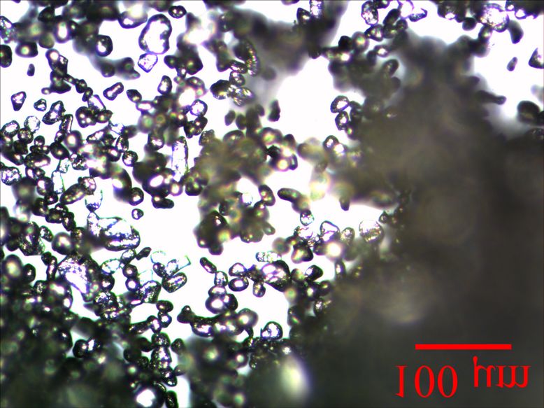
2                Bence G. Márkus et al.: Transport, Magnetic and Vibrational Properties of Chemically Exfoliated Few Layer Graphene

serious issue when one would like to apply bulk character-             quality the vibrational, electronic and transport properties
ization methods such as Electron Spin Resonance Spec-                  of the materials have to be investigated. We discuss the
troscopy (ESR) or macroscopic transport measurements                   Raman, ESR and microwave conductivity results.
(e.g. microwave conductivity). The substrate also has a
negative effect on the electronic and vibrational properties
of graphene (e.g. electronic interactions, various strains ap-
                                                                                                                                          G
ply). These effects are visible when one tries to compare
the results of free standing graphene [18] with graphene on                                                                                                                2D
                                                                                                                                                                                2

other substrates: [19] (Si-SiO2 ), [20] (Si-SiO2 and ITO),                                                                                                            2D
                                                                                                                                                                           1

                                                                                                                  D
[21] (SiC), [22] (glass).                                                                            e) Stirrer

    Other ways to create graphene in a mass production is
reduction from graphite/graphene oxide (GO) and wet
chemical exfoliation from graphite intercalation com-
pounds (GICs) with various solvents. Reduction process
is feasible in many chemical and biological routes with                                              d) Shear mixer

different quality of the final product [23–35]. In general,

                                                                         Raman Intensity (arb. u.)
the quality of final product may vary in a large scale but
always contains residual oxygen, missing carbon atoms,
free radicals, and dangling bonds therefore one can end up
with a thermally metastable material.                                                                c) Ultrasound

    Wet chemical or liquid phase exfoliation is the most
promising way to mass produce high quality materials
without disturbing the effects of the substrate [36–41]. For
the optimal quality of the outcome the effect of solvent [42]                                        b) SGN18
and the mechanical post procession has to be examined.
Here we report the transport, magnetic and vibrational
properties of Wet Chemically Exfoliated (WCEG) Few
Layer Graphene (FLG) using microwave conductivity,
electron spin resonance and Raman spectroscopies.
                                                                                                     a) HOPG

      2 Experimental We studied three WCEG species
which were prepared by different mechanical routes: ul-                                                1300   1350    1400   1500      1550   1600        1650 2600   2700          2800
trasounded (US), shear mixed (SM) and stirred (ST). All                                                                             Raman shift (cm )
                                                                                                                                                     -1

kinds were produced from saturate intercalated potassium
graphite powder, KC8 using DMSO solvent for wet exfo-
liation (full protocol described in Ref. [42]). The starting           Figure 1 D, G, 2D Raman modes of the investigated species us-
material, SGN18 graphite powder (Future Carbon) and                    ing 514 nm laser excitation. a) bulk HOPG, b) SGN18 graphite
Grade I bulk HOPG (SPI) were taken into comparison.                    powder, c) ultrasound sonicated exfoliated graphene, d) shear
Mechanical post processing were ultrasound treatment,                  mixed exfoliated graphene, e) stirred exfoliated graphene. Solid
shear mixing and magnetic stirring. The procedure was                  color line represents Lorentzian-fits, grey lines denotes the de-
done under argon atmosphere. The pristine materials were               composition of the 2D peaks. The dashed green line in case of
cleaned under high vacuum (10−7 mbar) at 400◦ C for one                the ultrasound sample points that the 2D peak can be fitted with
                                                                       one single Lorentzian as well.
hour to get rid of the remaining solvent and impurities. Ra-
man measurements were carried out in a high sensitivity
single monochromator LabRam spectrometer [43] using                        3.1 Raman spectroscopy Raman spectra of the ex-
514 nm laser excitation, 50× objective with 0.5 mW laser               amined samples are shown in Fig. 1. Namely, the D, G,
power. For ESR measurements a Bruker Elexsys E580                      and 2D Raman modes are shown. Solid lines represent
X-band spectrometer was used. Microwave conductiv-                     Lorentzian fits. In most cases 2D lines are made up of
ity measurements were done with the cavity perturbation                2 components, namely 2D1 and 2D2 . In the case of ul-
technique [44,45] extended with an AFC feedback loop to                trasound preparation the 2D feature can also be well fit-
increase precision [46]. The photographs were taken with               ted with one single Lorentzian. Parameters of the fitted
a Nikon Eclipse LV150N optical microscope using 5× (for                Lorentzian curves are given in Table 3.1.
FLG) and 10× (for SGN18) objectives.                                       Several observations can be made from the data in Ta-
                                                                       ble 3.1. one can make the following conclusions. The Ra-
   3 Results and Discussion To get an insight which                    man spectrum properties of graphite powder differs from
mechanical post production method produces the best                    HOPG. This is not an instrumental artifact, position and

Copyright line will be provided by the publisher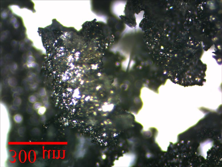
pss header will be provided by the publisher                                                                                                     3

width of peaks in case of graphite strongly depends on             2D2 mode can be interpreted as the presence of few layer
morphology and grain size [47].                                    sheets up to 4 layers. The width of the peaks suggest that
                                                                   we are dealing with single and few layer graphenes unlike
Table 1 Parameters of the fitted Lorentzian curves for the D, G,
                                                                   in turbostratic graphite (in that case the width of 2D would
and 2D Raman modes for a 514 nm excitation. ν denotes the po-      be about 50 cm−1 [19]). Bilayer graphene has a unique 2D
sition and ∆ν the FWHM in cm−1 , ∗ stands for single Lorentzian    peak made up of 4 components [19], which is not present
fit.                                                               here. In case of the ultrasounded sample, the 2D peak can
                                                                   also be well fitted with one single Lorentzian with a posi-
 514 nm     HOPG       SGN18       US        SM         ST
                                                                   tion up to 2715 cm−1 .
   νD       1358.4     1341.1    1355.5     1350.6    1353.9
                                                                       The intensity (amplitude) ratios of 2D and G peaks are
  ∆νD        18.6       15.5      20.0       29.4      14.2        given in Table 3.1.
   νG       1583.3     1570.3    1583.3     1581.6    1582.2
  ∆νG        6.9        8.1        9.5       10.6       9.6                                                                             ∗
                                                                   Table 2 Intensity (amplitude) ratios of 2D and G peaks,                  notes
  ν2D1      2688.4     2677.5    2702.9     2692.8    2692.4
                                                                   the single Lorentzian fit.
 ∆ν2D1       21.4       21.4      25.7       23.7      23.9
                                                                         514 nm      HOPG       SGN18       US         SM          ST
  ν2D2      2728.6     2714.1    2731.3     2726.1    2729.0
                                                                         I2D1 /IG     0.21       0.17      0.21        0.27       0.37
 ∆ν2D2       17.1       19.6      14.7       17.4      17.3
    ∗                                                                    I2D2 /IG     0.42       0.22      0.22        0.36       0.25
   ν2D                           2714.6
      ∗                                                                  I2D /IG      0.63       0.39      0.43        0.63       0.62
  ∆ν2D                            29.4                                     ∗
                                                                         I2D /IG                           0.24
     The D peak is less pronounced when ultrasound son-
ication or shear mixing was applied in case of exfoliated               Previous studies suggest that the number of layers can
graphenes. The position of the D peak varies between the           be extracted from this ratio [20, 48, 22]. Several other ef-
graphite powder and HOPG. According to mechanically                fect, including e.g. the effect of substrate (coupling-effect),
exfoliated and CVD studies [19, 12] the D peak is expected         the strain or compression, the method of the preparation,
at about 1350 cm−1 which is in a good agreement with               the type and quality of the solvent and the wavelength of
our results. Both Ferrari and Das [20] agrees that the in-         laser excitation also affects the 2D to G Raman signal ra-
tensity of the D peak for single layer material has to be          tio. Therefore the ratio of I2D /IG has to be treated with
small. The ultrasounded and shear mixed material satisfies         care. The ratio in case of mechanically exfoliated and CVD
this criterion. The D peak is always present in wet chemi-         samples on substrates is greater than one. For free stand-
cally exfoliated graphenes [38, 39] but its intensity is flake-    ing graphene and wet exfoliated species always lower than
size dependent [40]. The wet exfoliation according to the          one. Taking into account the previous considerations wet
D peak intensity is far better in quality than for reduced         exfoliated material is closer to free standing graphene than
GO samples [23,25,30].                                             the ones on substrates. The substrate may generate an ex-
     All our FLG samples have a sharp G peak very close            tra damping for the G band phonons, which can lower the
to HOPG (we remind that the starting material is SGN18).           intensity of the G peak therefore changes the ratio.
The width is about ∼ 2 cm−1 broader than graphite (both                 3.2 Electron Spin Resonance spectroscopy ESR
powder and bulk). Position of the G mode varies around             spectra of the investigated materials are presented in Fig.
1580 cm−1 in good agreement with previous studies [19,             2. All samples (including the SGN18 starting material)
20]. The G position also depends on the substrate and the          shows a narrow feature with a characteristic, uniaxial g-
number of layers. According to Ref. [18], the G peak po-           factor anisotropy lineshape, shown in the inset of Fig. 2.
sition for the shear mixed and ultrasounded materials are          This signal most probably comes from defects which are
very close to free standing graphene.                              embedded in the sp2 matrix of graphene. This would ex-
     The 2D peak for single layer graphene is expected to          plain the uniaxial nature of the g-factor anisotropy.
be a single, symmetric peak [19]. The position of the peak              The broader component for the SGN18 graphite sam-
is about 2700 cm−1 and shows a variation in the litera-            ple has a characteristic 12 mT ESR linewidth with a g-
ture [19, 20, 36,37]. Width of the peak also varies in a wide      factor of 2.0148 [49,50]. The line originates from conduct-
scale from 15 up to 40 cm−1 . Variations can be explained          ing electrons present in graphite, the value of g-factor is the
with the effect of the substrate (samples on substrates al-        weighted average of the two crystalline directions (B ∥ c
ways present a narrower peak) and the effect of prepara-           and B ⊥ c) with g-factors of the two, which are present
tions (strain, compressive forces may apply, chemicals may         in HOPG [51, 52, 49] with values of 2.0023 and 2.05. The
remain). Our FLG samples show two components for the               broader component has a 1.1 − 1.4 mT linewidth for the
2D line. The position of the lower 2D1 peak agrees with            three FLG samples with a g-factor slightly above the free-
previous single layer studies, thus this component is as-          electron value g0 = 2.0023. We tentatively assign this sig-
sociated with single layer graphene sheets. The 2D2 peak           nal to a few layer graphene phase which is p-doped due
position is close to that of graphite. The presence of the         to the solvent molecules. p-doping by e.g. AsF5 is known

                                                                                                   Copyright line will be provided by the publisher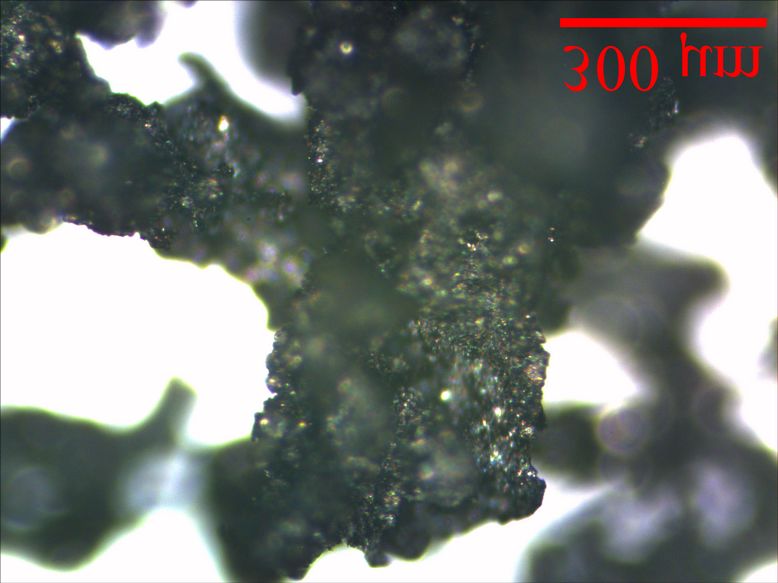
4 Bence G. Márkus et al.: Transport, Magnetic and Vibrational Properties of Chemically Exfoliated Few Layer Graphene
Table 3 g-factor, ∆B linewidth of the measured materials.
Broad component SGN18 US SM ST
g 2.0148 2.0059 2.0082 2.0094
ESR Intensity (arb. u.)
d) Stirrer
∆B (mT) 12.2 1.1 1.4 1.2
Narrow component SGN18 US SM ST
g g
||
g 2.0014 2.0013 2.0006 2.0013
351.6 352.0 352.4 352.8
Magnetic Field (mT) ∆B (mT) 0.08 0.04 0.04 0.04
ESR Intensity (arb. u.)
c) Shear mixer
Previous study done by Ciric [54] on mechanically ex-
foliated graphene showed a 0.62 mT wide peak with a g-
factor of 2.0045. On reduced GO [55] a g-factor of 2.0062
and a width of 0.25 mT was found. The solvothermally
synthesized graphene [56] shows a peak with a g-factor of
2.0044 and a width of 0.04 mT. According to these studies
b) Ultrasound wet exfoliated graphene species have a g-factor close to
reduced graphite, but with a width close to mechanically
exfoliated and solvothermally synthesized.
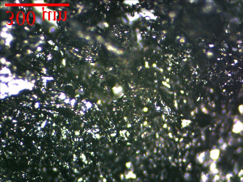
3.3 Microwave resistance Microwave resistance of
the investigated materials are presented in Fig. 3. This
method is based on measuring the microwave loss due
a) SGN18 to the sample inside a microwave cavity. This contactless
method is preferred when measuring resistance in powder
samples, however the measured loss depends on the sam-
ple amount and morphology. It therefore provides accurate
measurement of the relative temperature dependent resis-
340 345 350 355 360 365
tance, however it does not allow for a direct measurement
Magnetic Field (mT) of the resistivity. The resistance is proportional to the in-
verse of the microwave loss and it is normalized to that of
Figure 2 ESR spectra of a) SGN18 graphite powder, b) ultra- SGN18 at 25 K to get comparable results. Microscope im-
sounded, c) shear mixed, d) stirred FLGs. The graphite powder ages are presented as insets of Fig. 3. to demonstrate the
has a broad line of about 12.2 mTs as expected at a g-factor difference in grain size.
of 2.0148. Ultrasounded FLG present a Lorentzian of 1.1 mT All the measured materials have a semi-conducting be-
linewidth at g = 2.0059, the shear mixed present a 1.4 mT at havior in the investigated temperature range. This behavior
g = 2.0082. The stirred material has a uniaxial anisotropic line is usual to defective and inhomogeneous polycrystalline
with the width of 1.2 mT at g = 2.0094. The narrow uniaxial metals. The difference in the microwave loss in the dif-
anisotropic line is coming from defects and dangling bonds in all ferent samples is primarily due to a difference in the grain
cases. The inset shows the uniaxial g-factor simulated ESR line- size. The loss, L, is know to scale with the average grain
shape for the narrow component in the stirrer prepared sample. size as L = πB02 σR5 /5, where B0 is the amplitude of the
magnetic field, σ is the conductivity, and R is the average
radius of the grains [44, 57]. The average grain size was ob-
to give rise to similar signals with a g > g0 [53]. Ultra- tained as about 3−5 millimeters, 500 µm, and 300 microns
sounded and shear mixed materials present a single deriva- for the ultrasounded, stirred and shear mixed samples, re-
tive Lorentzian peak with a width of 1.1 mT and 1.4 mT, spectively, by analyzing the corresponding microscope im-
respectively. The stirred sample display a similar peak to ages. The trend in the microwave loss between the different
graphite powder, but with a much narrower width of 1.2 samples is thus found to follow the grain size.
mT. The g-factor of FLG materials is between the free elec-
tron and the graphite powders. The most probable explana- 4 Conclusions We studied the vibrational, magnetic
tion for this is that single layer sheets is giving a g-factor and transport properties of mechanically different post pro-
close to free electrons, but screened by the few layer sheets cessed few layer graphene systems with Raman, ESR spec-
whose g-factor is closer to graphite. The sharp lines are troscopy and microwave resistance measurements respec-
associated with the defects and dangling bonds. In all ma- tively. According to the results the difference in post pro-
terials the g-factor is below the free electrons 2.0023, thus cession does effect the investigated properties. From our
can be associated with p-type charge carriers. The spec- results one can figure out that ultrasound treatment ends
tra were simulated with derivative Lorentzian lineshapes up with the best results in a meaning that this is the closest
whose parameters are given in Table 3.2. to true single layer graphene.
Copyright line will be provided by the publisherpss header will be provided by the publisher 5
1.0 1.0
[9] S. Y. Zhou, G. H. Gweon, A. V. Fedorov, P. N. First, W. A.
de Heer, D. H. Lee, F. Guinea, A. H. C. Neto, and A. Lan-
zara, Nature Materials 6, 770 – 775 (2007).
0.9 0.9 [10] P. W. Sutter, J. I. Flege, and E. A. Sutter, Nature Materials
SGN18
7, 406 – 411 (2008).
[11] A. N. Obraztsov, E. A. Obraztsova, A. V. Tyurnina, and
0.8 0.8
A. A. Zolotukhin, Carbon 45, 2017–2021 (2007).
[12] A. Malesevic, R. Vitchev, K. Schouteden, A. Volodin,
Shear mixer L. Zhang, G. V. Tendeloo, A. Vanhulsel, and C. V. Hae-
0.7 0.7
sendonck, Nanotechnology 19, 305604 (2008).
(normalized to SGN18 at 25K)
[13] K. S. Kim, Y. Zhao, H. Jang, S. Y. Lee, J. M. Kim, K. S.
0.6 0.6
Kim, J. H. Ahn, P. Kim, J. Y. Choi, and B. H. Hong, Nature
Letters 457, 706–710 (2009).
[14] A. N. Obraztsov, Nature Nanotechnology 4, 212–213
0.5 0.5
(2009).
[15] A. Reina, X. Jia, J. Ho, D. Nezich, H. Son, V. Bulovic,
M. S. Dresselhaus, and J. Kong, Nano Letters 9(1), 30–35
0.4 0.4 (2009).
[16] C. Mattevi, H. Kima, and M. Chhowalla, Journal of Mate-
-1
rials Chemistry 21, 3324–3334 (2011).
L
0.3 0.3
[17] Q. Yu, L. A. Jauregui, W. Wu, R. Colby, J. Tian, Z. Su,
Ultrasound
H. Cao, Z. Liu, D. Pandey, D. Wei, T. F. Chung, P. Peng,
N. P. Guisinger, E. A. Stach, J. Bao, S. S. Pei, and Y. P.
0.2 0.2
Stirrer
Chen, Nature Materials 10, 443–449 (2011).
[18] C. C. Chen, W. Bao, J. Theiss, C. Dames, C. N. Lau, and
0.1 0.1
S. B. Cronin, Nano Letters 9(12), 4172–4176 (2009).
[19] A. C. Ferrari, J. C. Meyer, V. Scardaci, C. Casiraghi,
M. Lazzeri, F. Mauri, S. Piscanec, D. Jiang, K. S.
Novoselov, S. Roth, and A. K. Geim, Physical Review Let-
5 10 15 20 25 50 100 150 200 250
Temperature (K)
ters 97, 187401 (2006).
[20] A. Das, B. Chakraborty, and A. K. Sood, Bull. Mater. Sci.
31(3), 579–584 (2008).
Figure 3 Microwave resistance of FLGs compared to graphite. [21] C. Faugeras, A. Nerriere, and M. Potemski, Applied
Insets are microscope images from the materials. Note the differ- Physics Letters 92, 011914 (2008).
ent scale for the SGN18 graphite sample. The different resistance [22] J. Tsurumi, Y. Saito, and P. Verma, Chemical Physics Let-
of FLG species can be explained with the different grain size. ters 557, 114–117 (2013).
[23] C. Gomez-Navarro, R. T. Weitz, A. M. Bittner, M. Scolari,
A. Mews, M. Burghard, and K. Kern, Nano Letters 7(11),
Acknowledgements Work supported by the European Re- 3499–3503 (2007).
search Council Grant No. ERC-259374-Sylo. [24] Z. Osváth, A. Darabont, P. Nemes-Incze, E. Horváth, Z. E.
Horváth, and L. P. Biró, Carbon 45, 3022–3026 (2007).
References [25] S. Stankovich, D. A. Dikin, R. D. Piner, K. A. Kohlhaas,
[1] H. W. Kroto, J. R. Heath, S. C. O’Brien, R. F. Curl, and A. Kleinhammes, Y. Jia, Y. Wu, S. T. Nguyen, and R. S.
R. E. Smalley, Nature 318, 162 – 163 (1985). Ruoff, Carbon 45, 1558–1565 (2007).
[2] S. Iijima, Nature 354, 56 – 58 (1991). [26] G. Eda, G. Fanchini, and M. Chhowalla, Nature Letters 3,
[3] K. S. Novoselov, A. K. Geim, S. V. Morozov, D. Jiang, 270–274 (2008).
Y. Zhang, S. V. Dubonos, I. V. Grigorieva, and A. A. Firsov, [27] S. Park and R. S. Ruoff, Nature Nanotechnology 4, 217–
Science 306, 666–669 (2004). 224 (2009).
[4] A. K. Geim and K. S. Novoselov, Nature Materials 6, 183 [28] D. R. Dreyer, S. Park, C. W. Bielawski, and R. S. Ruoff,
– 191 (2007). Chemical Society Reviews 39, 228–240 (2010).
[5] A. K. Geim, Science 324, 1530–1534 (2009). [29] Y. Shao, J. Wang, M. Engelhard, C. Wang, and Y. Lin, Jour-
[6] A. H. C. Neto, F. Guinea, N. M. R. Peres, K. S. Novoselov, nal of Materials Chemistry 20, 743–748 (2010).
and A. K. Geim, Reviews of Modern Physics 81, 109–162 [30] J. Zhang, H. Yang, G. Shen, P. Cheng, J. Zhang, and
(2009). S. Guo, Chem. Commun. 46, 1112–1114 (2010).
[7] B. Jayasena and S. Subbiah, Nanoscale Research Letters [31] W. Chen, L. Yan, and P. R. Bangal, Carbon 48, 1146–1152
6(1), 95 (2011). (2010).
[8] C. Berger, Z. Song, X. Li, X. Wu, N. Brown, C. Naud, [32] W. Chen, L. Yan, and P. R. Bangal, J. Phys. Chem 114,
D. Mayou, T. Li, J. Hass, A. N. Marchenkov, E. H. Con- 19885–19890 (2010).
rad, P. N. First, and W. A. de Heer, Science 312, 1191–1196 [33] S. Pei, J. Zhao, J. Du, W. Ren, and H. M. Cheng, Carbon
(2006). 48, 4466 –4474 (2010).
Copyright line will be provided by the publisher6 Bence G. Márkus et al.: Transport, Magnetic and Vibrational Properties of Chemically Exfoliated Few Layer Graphene
[34] E. C. Salas, Z. Sun, A. Lüttge, and J. M. Tour, Carbon 48, [56] B. Náfrádi, M. Choucair, and L. Forró, Carbon 74, 346–
4466 –4474 (2010). 351 (2014).
[35] S. Pei and H. M. Cheng, Carbon 50, 3210 –3228 (2012). [57] H. Kitano, R. Matsuo, K. Miwa, A. Maeda, T. Takenobu,
[36] Y. Hernandez, V. Nicolosi, M. Lotya, F. M. Blighe, Z. Sun, Y. Iwasa, and T. Mitani, Phys. Rev. Letters 88(9), 096401
S. De, I. T. McGovern, B. Holland, M. Byrne, Y. K. (2002).
Gun’ko, J. J. Boland, P. Niraj, G. Duesberg, S. Krishna-
murthy, R. Goodhue, J. Hutchison, V. Scardaci, A. C. Fer-
rari, and J. N. Coleman, Nature Nanotechnology 3, 563–
568 (2008).
[37] J. M. Englert, J. Roöhrl, C. D. Schmidt, R. Graupner,
M. Hundhausen, F. Hauke, and A. Hirsch, Adv. Mater. 21,
4265–4269 (2009).
[38] M. Lotya, Y. Hernandez, P. J. King, R. J. Smith, V. Ni-
colosi, . S. Karlsson, F. M. Blighe, S. De, Z. Wang, I. T. Mc-
Govern, G. S. Duesberg, and J. N. Coleman, J. Am. Chem.
Soc. 131, 3611–3620 (2009).
[39] J. M. Englert, C. Dotzer, G. Yang, M. Schmid, C. Papp,
J. M. Gottfried, H. P. Steinrück, E. Spiecker, F. Hauke, and
A. Hirsch, Nature Chemistry 3, 279–286 (2011).
[40] J. Coleman, Accounts of Chemical Research (2013).
[41] A. Hirsch, J. M. Englert, and F. Hauke, Accounts of Chem-
ical Research 1, 87–96 (2013).
[42] P. Vecera, J. C. Chacón-Torres, S. Reich, F. Hauke, and
A. Hirsch, handout (2015).
[43] G. Fábián, C. Kramberger, A. Friedrich, F. Simon, and
T. Pichler, Review of Scientific Instruments 82, 023905
(2011).
[44] O. Klein, S. Donovan, M. Dressel, and G. Grüner, Inter-
national Journal of Infrared and Millimeter Waves 14(12),
2423–2456 (1993).
[45] S. Donovan, O. Klein, M. Dressel, K. Holczer, and
G. Grüner, International Journal of Infrared and Millimeter
Waves 14(12), 2459–2487 (1993).
[46] B. Nebendahl, D. N. Peligrad, M. Pozek, A. Dulcic, and
M. Mehring, Review of Scientific Instruments 72, 1876–
1881 (2001).
[47] Y. Wang, D. C. Alsmeyer, and R. L. McCreery, Chem.
Mater. 2, 557–563 (1990).
[48] Z. H. Ni, T. Yu, Z. Q. Luo, Y. Y. Wang, L. Liu, C. P. Wong,
J. Miao, W. Huang, and Z. X. Shen, ACS Nano 3(3), 569 –
574 (2009).
[49] D. L. Huber, R. R. Urbano, M. S. Sercheli, and C. Rettori,
Phys. Rev. B 70, 125417 (2004).
[50] M. Galambos, G. Fábián, F. Simon, L. Ćirić, L. Forró,
L. Korecz, A. Rockenbauer, J. Koltai, V. Zólyomi,
A. Rusznyák, J. Kürti, N. M. Nemes, B. Dóra, H. Peter-
lik, R. Pfeiffer, H. Kuzmany, and T. Pichler, Phys. Status
Solidi B 246(11–12), 2760–2763 (2009).
[51] M. Sercheli, Y. Kopelevich, R. R. da Silva, J. H. S. Torres,
and C. Rettori, Physica B 320, 413–415 (2002).
[52] M. Sercheli, Y. Kopelevich, R. R. da Silva, J. H. S. Torres,
and C. Rettori, Solid State Communications 121, 579–583
(2002).
[53] M. S. Dresselhaus and G. Dresselhaus, Advances in
Physics 30, 1–186 (1981).
[54] L. Ćirić, A. Sienkiewicz, B. Náfrádi, M. Mionić, A. Ma-
grez, and L. Forró, Phys. Status Solidi B 246(11–12),
2558–2561 (2009).
[55] L. Ćirić, A. Sienkiewicz, R. Gaál, J. Jaćimović, C. Vâju,
A. Magrez, and L. Forró, Phys. Rev. B 86, 195139 (2012).
Copyright line will be provided by the publisherYou can also read