Two-Phase Flow Phenomena in Gas Turbine Compressors with a Focus on Experimental Investigation of Trailing Edge Disintegration - MDPI
←
→
Page content transcription
If your browser does not render page correctly, please read the page content below
aerospace
Article
Two-Phase Flow Phenomena in Gas Turbine Compressors
with a Focus on Experimental Investigation of Trailing
Edge Disintegration
Adrian Schlottke *             and Bernhard Weigand

                                          Institute of Aerospace Thermodynamics, University of Stuttgart, 70569 Stuttgart, Germany;
                                          bernhard.weigand@itlr.uni-stuttgart.de
                                          * Correspondence: adrian.schlottke@itlr.uni-stuttgart.de; Tel.: +49-711-685-62321

                                          Abstract: Two-phase flow in gas turbine compressors occurs, for example, at heavy rain flight condi-
                                          tion or at high-fogging in stationary gas turbines. The liquid dynamic processes are independent
                                          of the application. An overview on the processes and their approach in literature is given. The focus
                                          of this study lies on the experimental investigation of the trailing edge disintegration. In the experi-
                                          ments, shadowgraphy is used to observe the disintegration of a single liquid rivulet with constant
                                          liquid mass flow rate at the edge of a thin plate at different air flow velocities. A two side view enables
                                          calculating droplet characteristics with high accuracy. The results show the asymptotic behavior
                                          of the ejected mean droplet diameters and the disintegration period. Furthermore, it gives a de-
                                          tailed insight into the droplet diameter distribution and the spreading of the droplets perpendicular
                                          to the air flow.

                                   Keywords: two-phase flow; trailing edge disintegration; gas turbine compressor
Citation: Schlottke, A.; Weigand, B.
Two-Phase Flow Phenomena in Gas
Turbine Compressors with a Focus on
Experimental Investigation of Trailing    1. Introduction
Edge Disintegration. Aerospace 2021,            Two-phase flow in gas turbine compressors occurs e.g., at heavy rain flight conditions
8, 91. https://doi.org/10.3390/           or in high-fogging applications. The liquid dynamic processes can be categorized into
aerospace8040091                          four major processes. All of them are shown in Figure 1. In the following, the processes
                                          will shortly be stated, followed by a more detailed description of the processes within
Academic Editor: Lakshmi N. Sankar
                                          each regime. Literature findings will be cited to show the state-of-the-art understanding
                                          of the processes and their modeling. In flight conditions, as well as in high-fogging in sta-
Received: 25 February 2021
                                          tionary gas turbines, many polydisperse droplets are present, with diameter distributions
Accepted: 23 March 2021
                                          in the range of 10 to 200 µm [1]. The first process accounts for single droplet interaction
Published: 26 March 2021
                                          with the air flow and the influence of polydisperse spray. As soon as the droplets en-
                                          ter the compressor, interactions with the compressor parts are inevitable, where mainly
Publisher’s Note: MDPI stays neutral
                                          the compressor blades will be hit by droplets as they are redirecting the flow. This curvature
with regard to jurisdictional claims in
                                          of the streamlines cannot be followed by droplets of all size due to inertia effects and thus
published maps and institutional affil-
iations.
                                          droplets impact onto the compressor blade surface. Depending on the incidence angle
                                          α, impact is possible on the pressure and the suction side. The question arises whether
                                          the droplet stays attached onto the surface, or if it is rejected back into the air flow or a com-
                                          bination of both. The subsequent wetting of the compressor blade surface through sticking
                                          droplets is another major process, which can be subdivided into wall film motion, wall
Copyright: © 2021 by the authors.
                                          film breakup and rivulet flow. The last process is the trailing edge disintegration. Driven
Licensee MDPI, Basel, Switzerland.
                                          by the shear of the gas flow, the liquid reaches the trailing edge of the compressor blade
This article is an open access article
                                          and disintegrates into ligaments and droplets. At this point, the processes will start over
distributed under the terms and
                                          again, as the outcoming droplets from the first compressor row are penetrating towards
conditions of the Creative Commons
Attribution (CC BY) license (https://
                                          the second row and so on.
creativecommons.org/licenses/by/
4.0/).

Aerospace 2021, 8, 91. https://doi.org/10.3390/aerospace8040091                                           https://www.mdpi.com/journal/aerospace
Aerospace 2021, 8, 91 2 of 15
Figure 1. Scheme of the main liquid dynamic processes occurring at two-phase flow in gas turbine
compressors. Reproduced with the permission from H. Gomaa, Modeling of Liquid Dynamics in
Spray Laden Compressor Flows; published by Verlag Dr. Hut, 2014. [2].
To highlight the importance of this article for the completeness of understanding all
of the processes, their appearance in literature is given in the following. First, droplets
and spray are considered. The relative velocity between gas and droplet leads to a de-
formation of the droplet. If the relative velocity is high, the droplet can break up into
smaller fractions. There exist several publications regarding droplets in accelerated air flow,
which characterize the outcome. A detailed description of droplet breakup mechanisms
can be found in [3]. Droplets with D ≥ 100 µm can reach the bag breakup regime, which is
experimentally investigated in [4].
Impact on the compressor blade surface is mainly observed for droplets with
D ≥ 30 µm. This can be explained by their relaxation behavior. Analytic estimations
considering drag of the droplets show that the limit for perfect relaxation within the char-
acteristic length of a compressor blade lies at D ≈ 25 µm [5]. Thus, larger droplets are
not able to follow the curved streamlines around the compressor blade and thus might
hit the surface. The phenomena of droplet impact onto dry and wetted walls has been
investigated by many authors in literature. Although more possible outcomes exist when
a droplet hits a wall, for the application of two-phase-flow in gas turbine compressors,
only the distinction between deposition and splashing into a number of secondary droplets
is of interest. In [6], a splashing criteria is given for droplet impact on dry surfaces and
in [7] for wetted surface depending on the liquid film height, respectively. The existence
of a liquid film affects not only the splashing limit, but also the splashing outcome. It
is possible that more liquid mass is ejected into the air flow than the impacting droplet
mass itself. Therefore, the modeling of droplet impact and its outcome play a major role
in the prediction of the arising liquid wall film. To gain insight in the deposited liquid
mass and the secondary droplet spectrum which is ejected back into the air flow, direct
numerical investigations of single droplet impact validated with experimental data were
performed in [2,8]. Another approach is to use empirical correlations, as in [6], for single
droplet impact on dry walls or in [9] for single droplet impact on shear driven liquid wall
films.
If enough liquid mass is deposited on the compressor blade surface, a thin wall film is
created. The air flow drives the liquid wall film towards the trailing edge through shear
stress. At the pressure side, a closed wavy film runs down the compressor blade. Here,
the film is quite stable, as droplet impact occurs continuously over the pressure side. This
is mainly due to its concave shape [1]. In contrast, on the suction side, droplet impact is
only visible within a short region from the leading edge. As soon as the stabilizing effect
of droplet impact ceases, the wall film is sensitive to instabilities. In many cases, the thin
wall film breaks up into rivulets. The breakup position, the number of rivulets, as well as
their height and width, were experimentally investigated in [1] and an empirical approach
to calculate the wall film height is given. Simulations of the liquid wall film under the same
conditions using simplified incompressible Navier–Stokes equations were performed in [2].
Simplifications were possible due to the small aspect ratio between film height and blade
length. Both methods were capable of reproducing the experimental data qualitativelyAerospace 2021, 8, 91 3 of 15
well. Recently, the breakup of shear driven films and the consecutive movement of rivulets
has been analyzed experimentally and analytically in [10].
At the trailing edge, the liquid accumulates and disintegrates periodically. Due
to the breakup of the wall film, only separated rivulets reach the trailing edge. In literature,
atomization is widely investigated because of its wide field of applicability (combustion,
painting, spray cooling, etc). However, research focused mainly on atomization with
the use of nozzles or liquid jets and sheets. An overview is given in [11–13]. One type
of nozzle is using a similar method for atomization: prefilm atomizers. Here, the liquid
forms a thin film on a wall, driven towards the trailing edge by the concurrent gas flow,
where it disintegrates into droplets. In [14], the column-wise disintegration at a prefilmer’s
trailing edge is shown and the disintegration of each rivulet is assumed to be independent.
Additional information on the influence of ambient pressure and film loading on the ejected
droplet spectrum is given in [15]. However, findings from prefilm atomizers cannot di-
rectly be adopted to the disintegration at the trailing edge of a compressor blade. This
ensues from the geometrical dimensions, as the ratio between prefilmer length and channel
height are much smaller compared to gas turbine applications. Therefore, the top wall
may influence the boundary layer in prefilm atomizers. First, experimental investigations
on trailing edge disintegration in conditions comparable to gas turbines were performed
in [16] and continued in [17], with a focus on the droplet size, acceleration and disinte-
gration time. More recently, Refs. [18,19] investigated the effect of the trailing edge size
and the angle of attack on the disintegrated droplet characteristics. Ref. [2] investigated
the disintegration of a single liquid rivulet at the trailing edge of a thin plate. The goal
of the cited work was to gain integral insight in the disintegration process, thus to be able
to put up a model for numerical investigations.
This manuscript shall continue the work done in [2]. Instead of using a superhy-
drophobic surface, a thin acrylic glass (PMMA) plate is used. In addition, the observation
area is increased to be able to observe the complete disintegration process, even for larger
ligaments. The focus lies on a more detailed description of the disintegration process. This
includes the comparison of the whole droplet diameter distribution and their evolution
instead of mean values, investigation of ligament length scales at the instance of disintegra-
tion and their time scales. In particular, the length scales of ligaments are an interesting
feature in gas turbine compressors. It determines if a secondary breakup can take place
until the next compressor stage is reached, or if even the ligament will hit the next stage.
2. Materials and Methods
The following experiments are performed in a flow channel with quadratic cross section
with an edge length of 80 mm. The inlet of the flow channel is a nozzle with an area ratio
of 31.6. The nozzle is followed by a section with constant cross section with a length of 6.0 m.
At the end of the flow channel a diffusor with an area ratio of 2.8 is used to connect the channel
to the compressor, which is used in suction mode. The compressor is controlled via the ro-
tational frequency and the maximum volume flow rate can be adjusted by using a throttle
valve. Within this experimental campaign, only about 50% of the maximum volume flow rate
is used, as it is sufficient to reach the designated velocity range of 10–38 m/s and, therefore,
the adjustability of the compressor is higher. The Reynolds number of the air flow ReG is in
the range of 12,900–45,600, where
ρG uG L
ReG = . (1)
µG
In Equation (1), ρ is the density, u the velocity, L is the characteristic length, and µ is
the dynamic viscosity. The experimental setup parameters are given in Table 1.The length
of the thin plate L = 20 mm is chosen as a characteristic length for the ReG number. The
prevailing velocity during the experiment is measured with a Prandtl probe 1.25 m down-
stream from the probe position. Within this velocity range, the three main disintegrationAerospace 2021, 8, 91 4 of 15
regimes can be observed. These are defined analogous to the breakup processes of liquid
jets [20]: symmetric and asymmetric Rayleigh breakup and bag breakup.
Table 1. Parameters of the experimental test campaign.
Liquid Mass Flow Rate (g/h) 900
Air flow velocity (m/s) 10.5 13.3 15.3 16.7 18.4 19.8 21.4 22.7 23.9
ReG 12,930 16,640 18,999 20,737 23,051 25,022 26,809 28,188 29,678
Air flow velocity (m/s) 24.6 26.0 27.2 28.3 29.1 30.3 31.0 31.6 32.7
ReG 30,277 32,571 34,374 34,831 35,815 37,625 38,154 38,892 40,246
Air flow velocity (m/s) 33.9 34.7 35.1 36.1 36.8 37.4
ReG 41,723 42,326 42,814 44,034 44,888 45,620
The test section position is 3.21 m from the nozzle exit, which gives an entrance
length of 40.1 hydraulic diameters, after which a fully developed turbulent flow can
be assumed [21]. The thin PMMA plate with a length of L = 20 mm and a thickness
of t p = 20 µm is mounted horizontally in the center of the channel. To ensure that
disintegration takes place in the focus plane, the rivulet is guided to the trailing edge in
a straight line. This is done by putting a hydrophobic coating on the sides of the PMMA
plate, leaving a small gap in the middle for the rivulet with a width of 1 mm. The apparent
contact angle of the two surfaces are θ app = 80.4◦ for PMMA and θ app = 105.2◦ for
the hydrophobic surface. The liquid is supplied through a capillary needle, which enters
the flow channel from above and has an inner diameter of Din = 0.6 mm and an outer
diameter of Dout = 0.91 mm. Its tip is close to the thin plate surface, to ensure that the liquid
deposits on the surface without splashing and a less possible disturbance. The liquid mass
flow is controlled via a Coriolis mass flow controller (Bronkhorst Deutschland Nord GmbH,
59174 Kamen, Germany).
The observation of the disintegration process is done optically, using shadowgraphy.
The optical setup is shown in Figure 2, where all parts and the dimensions of the thin
plate are labeled and the global coordinate system, with the origin at the trailing edge,
is shown. The pictures are lit by a LED on each side and the light is paralellized using
plano-convex lenses to gain more brightness and reach uniform background lighting. The
top and side view are captured with one camera. Therefore, the optical setup contains two
silver-coated mirrors and one semi-transparent mirror. All mirrors are movable with six
degrees of freedom to be able to adjust the light path and optimize the captured image.
To focus the image on the camera, a lens with a fixed focal length of f = 150 mm was used.
The aperture was closed as much as possible to gain a large depth of field. This is important,
as the disintegration produces ligaments and droplets that fill the whole captured area. A
high speed camera (PHOTRON SA1.1) is used at a full resolution of 1024 × 1024 pixels
with a maximum frame rate of 5400 fps, which is needed to capture the high frequencies
of the disintegration process. Additionally, when bag breakup occurs, small droplets are
catapulted from the lamella at high speeds. To capture this without blur, the shutter speed
is set to 1/62,000 s. 8 bit greyscale images are used and the scale of the image is 38.9 µm
pixel for top and side view. The image is split unequally for top and side view with a ratio
of 2:3, as the disintegration processes, mainly the bag breakup, takes place over a larger
area in the side view than in the top view. The top view is in the upper part of the image,
whereas the side view is in the lower part. Together with the scale, this gives a field of view
for the top view of 39.8 × 23.9 mm2 and for the side view of 39.8 × 15.9 mm2 . With these
preferences, the high speed camera is able to capture 10, 928 frames, which equals a time
interval of about 2 s. As shown later, the disintegration period decreases with growing gas
velocity. This means that, for the same time interval, more disintegrations occur. For statis-
tical measures, it is important to have a sufficiently large number of disintegrated droplets.
Therefore, the experimental cases at velocities vG ≤ 15.3 m/s are repeated two or threeAerospace 2021, 8, 91 5 of 15
times to gain a larger database and therefore reduce uncertainty.
ṁ L 2 1
1 Semitransparent Mirror
5
2 Mirror 3
4
3 Lense z
x
4 LED
y
5 Needle tp L 2
6
6 Thin plate
uG 3
4
Figure 2. Sketch of the experimental setup with a focus on the optical setup. The objective
and the high speed camera are omitted. The light path for top (green) and side view (red) are
depicted with dashed lines.
In the following, the routine to evaluate the single images will shortly be discussed.
The complete evaluation is performed using MATLAB R2020a (The MathWorks Inc., Natick,
MA, USA.) As mentioned before, shadowgraphy is used in the experiments. At the begin-
ning of each experiment a background picture is taken, where no liquid is visible. From this
picture, the position of the trailing edge can be evaluated. In the first step of the evaluation,
each frame is subtracted from the background, which leaves only the liquid structures
visible and all background structures and most noise are removed. These differential
images are then split into top and side view. The images need to be binarized to evaluate
the properties of the visible structures. The threshold to perform the binarization is evalu-
ated separately for the top and side view. To also account for slightly changing brightness
intensity between the experiments, the threshold is evaluated for each experiment sepa-
rately. To set the threshold value, one image of each series containing an exposed droplet is
used. The droplet should be large in comparison to its image series. The threshold is then
defined as the mean of the inflection points’ gray value of straight lines through the droplet
center. An intrinsic routine gathers the properties of the structures in the binarized image,
such as area, centroid, eccentricity and the equivalent diameter, which is stored for each
image. The equivalent diameter is defined as the diameter of a circle having the same
area as the identified liquid structure. A filtering routine removes very small structures,
which arise from remaining noise and also identifies the ligament which is connected
to the trailing edge. The evaluation of the disintegration period is done semi-automatically,
where one period is defined as the disintegration of a connected ligament. Figure 3 shows
the disintegration process at two different gas velocities. The corresponding ReG number
is given in the image. At low gas velocities, disintegration is easily distinguishable, as
the time between two disintegrations is large enough for droplets to be transported out
of the observed area. With increasing gas velocities, the process reaches higher frequencies,
which leads to overlapping disintegrations, so the droplets of the previous disintegration
are not transported out of the observed area, before the following disintegration begins.
This makes an automation difficult. Therefore, the routine detects possible disintegration
time frames depending on the ligament length touching the trailing edge and the num-
ber of droplets close to the trailing edge. The method is implemented conservatively,
to assure that all disintegrations are recognized. Excess frames where no disintegration
occurs are manually removed. After knowing the disintegration frames, the data for each
disintegration can be evaluated in a statistical manner.Aerospace 2021, 8, 91 6 of 15
Figure 3. Typical disintegration process at two different gas velocities and ReG numbers, respectively.
Both images show top and side view. The thin plate and with it the trailing edge is visualized with
the grey area. The dashed lines show the positions, where the droplets are counted.
Due to the high-speed imaging, several images are taken of the same disintegration. In
order to not account for the same droplets multiple times, the droplets are counted at two
positions, which are highlighted in Figure 3 with dashed lines. Position A has a distance
of 600 pixel (23.3 mm) from the trailing edge and position B a distance of 900 pixel
(35.0 mm), respectively. With the count at the two positions, changes due to secondary
breakup can be estimated. The estimation of the droplet parameters is done in parallel
for the top and side view and matched together in the end. In this way, not only planar,
but spatial information can be evaluated for each droplet. Therefore, the volume can be
calculated with higher accuracy and with it derived quantities like the equivalent diameter.
3. Results and Discussion
This section is divided into four parts. The parts describe the different stages on
the travel from the rivulet at the trailing edge, over the disintegration process itself
to the developed spray and the deviation of the trajectories of the droplets. The first
part covers the liquid rivulet and the ligament which is connected to the trailing edge.
Second, the disintegration process itself is characterized. Here, the disintegration period
and the disintegrated volume are evaluated. Third, the ejected droplets are characterized.
The focus lies on the droplet diameter and its distribution depending on the ambient condi-
tions. The last part deals with the droplet trajectories, more precisely with the spreading
perpendicular to the air flow direction.
3.1. Rivulet and Ligament Characteristics
In the following, the characteristics of the liquid rivulet and the ligament which still
touches the trailing edge are discussed in detail. The evaluated image always shows
the trailing edge of the thin plate, which makes the evaluation of rivulet parameters
possible. With the two side view, the height and the width of the rivulet can be measured.
Both measurements are performed directly at the trailing edge. The third parameter
of interest is the length of the ligament, which still touches the trailing edge. The length
is defined as the horizontal distance between the trailing edge and the farthest point
of the ligament. Over time, all three parameters are fluctuating periodically, which can
be explained by mass conservation. The mass flow controller provides a constant mass
flow rate, which is transported to the trailing edge. As the disintegration process is
discontinuous, but occurs periodically, liquid accumulates at the trailing edge, which
leads to an increase of rivulet width and height. At some point, the liquid starts to flow
over the trailing edge and a ligament develops. While this ligament is growing, widthAerospace 2021, 8, 91 7 of 15
and height of the rivulet at the trailing edge are already decreasing. As soon as the ligament
disintegrates, only a small portion remains at the trailing edge and the cycle starts all over.
To compare the three parameters for different ReG numbers, mean values will be calculated.
This is done by using arithmetic mean values x. In addition, the standard deviation S is
calculated with
v
N
u
u 1
S=t ∑ ( x − x )2 .
N − 1 i =1 i
(2)
The number of evaluated data points xi is N. For the rivulet height and width, all
values in each experimental test case are used. For the maximum ligament length, only
the values one frame before the ligament disintegrates are used.
Figure 4 shows the evolution of the three parameters depending on the air flow ReG
number. The dashed lines are the mean values, where the dots show the ReG numbers
where measurements were taken. The colored area shows the standard deviation S. First,
we want to look at the rivulet width (colored in blue). It takes values from 2.0 mm
at ReG = 38, 890 up to 4.2 mm at ReG = 20, 740. However, it is quite constant for a wide
range of ReG numbers with a width of about 2.7 mm. It is also apparent that the standard
deviation is nearly independent of the ReG number and has a value of about S = 0.9 mm.
If we now look at the rivulet height, a monotonous decrease is visible. This can be explained
by mass conservation. As ReG of the air flow increases, the shear stress at the liquid surface
increases. Respectively, the velocity of the rivulet will increase. Thus, with constant
width, the height has to reduce to get a smaller cross section to fulfill mass conservation.
The standard deviation is also decreasing for larger ReG numbers. Finally, the ligament
length Llig at the instance of disintegration will be discussed. It shows an interesting
behavior, as it is first strongly increasing with ReG showing a maximum at ReG = 19, 000.
Figure 4. Characteristics of the ligament connected to the trailing edge plotted over the Reynolds number of the air flow.
The dashed lines show the mean values. The colored areas show the standard deviation.
After that, it decreases slowly until it reaches approximately the same value as for
low ReG numbers. The standard deviation is large for low ReG numbers with up to 28%.Aerospace 2021, 8, 91 8 of 15
However, after the maximum value of Llig , the standard deviation is reducing to 17%.
The non monotonous behavior of Llig can be explained by a change in the disintegration
process. At the point of maximum ligament length, the transition from asymmetric Rayleigh
breakup towards bag breakup takes place. The air flow velocity is high enough to transport
the liquid ligament far downstream, before the Rayleigh instabilities force a breakup
of the ligament into droplets. On the other side, the air flow velocity is low enough, so
that liquid surface tension is able to keep the ligament together. This is in contrast to high
air flow velocities, where liquid bags are also created; however, they are immediately
disintegrated into separate droplets.
3.2. Disintegration
Disintegration occurs periodically at the trailing edge. Two main characteristics will
be evaluated in the following: the disintegration period and the disintegrated volume.
The disintegration period is defined in this context as the time between the beginning of two
consecutive disintegrations. The disintegrated volume is the corresponding volume of all
droplets that disintegrates from the trailing edge within that time frame. As mentioned
above, the definition of a disintegration is easy for low ReG numbers, as the droplets
of each disintegration are transported out of the evaluation area, before the next one starts.
In the case of overlapping disintegrations, one disintegration is defined as one flapping
of the ligament, as can be seen in Figure 3 at ReG = 44,034.
To describe the disintegration period depending on the ReG number, two effects shall
be discussed. On one side, the influence on the mean disintegration period and on the other
side, the influence on the variation of the disintegration period. In Figure 5, the cumulative
distribution function (CDF) of the disintegration time period for different ReG numbers is
shown. From the CDF, different results can be seen. The shift of the colored areas from right
to left shows that, with increasing ReG number, the average disintegration period tends
to smaller values. This shift follows an asymptotic behavior, as the difference is getting
smaller for increasing ReG numbers. The averaged disintegration period tends to a finite
minimum value of about 0.006 s.
Figure 5. Cumulative distribution function of the disintegration time period at varied ReG number. Each colored area
belongs to one ReG number, indicated by the text inside the area.Aerospace 2021, 8, 91 9 of 15
It needs to be mentioned that the CDF is not shown for every ReG number from the ex-
periments. This is due to the asymptotic behavior. For ReG > 37,625, the different CDF lie
so close together that an optical distinction is no longer possible. From the CDF, statements
on the distribution can also be made. The width between the points, where the CDF have
the values of 0 and 1, states which disintegration periods were visible in the experiments. The
slope at a distinct time value is proportionally linked to the probability of this value. Again,
for an increasing ReG number, the width is decreasing and the slopes are increasing. This
shows that not only is the variability of disintegration times smaller for higher ReG numbers,
but also the probability of disintegration times apart from the mean value.
The disintegrated volume is strongly coupled to the disintegration period, as the mass
flow rate towards the trailing edge is fixed. Therefore, it is assumed that the disintegrated
volume shows the same asymptotic behavior as the disintegration period. This can be
seen in Figure 6. The dashed line in the blue area shows the mean disintegration volume.
To get the average, the disintegrated volume at every disintegration and the total number
of disintegrations observed were evaluated. The blue area shows the standard deviation
calculated with Equation (2). The behavior confirms the above stated assumption. With
increasing ReG numbers, the disintegration volume decays asymptotically to a value
of 1.3 mm3 . The same findings apply for the standard deviation.
Figure 6. Mean disintegrated volume and mean D10 plotted depending on the ReG number. Dashed lines show the mean
values, the circles indicate the measurement points, and colored areas show the standard deviation.
3.3. Droplets and Spray
At the instance of disintegration, one ligament contains the whole disintegrated
volume for the cases where no bag breakup occurs. With time, this ligament further dis-
integrates into smaller droplets due to surface tension and shear stress through the outer
air flow. If bag breakup occurs, the thin film of the bag ruptures and many small droplets
are ejected before the ligament disintegrates from the trailing edge. The resulting spray
of droplets will be characterized in the following two ways. First, an integral view by
comparing the mean droplet diameter D10 will be given. This can be seen in Figure 6.
The dashed line corresponding to the green area shows the average D10 of all disintegra-
tions within one experiment. The area represents the standard deviation calculated with
Equation (2). The overall behavior of D10 also follows an asymptotic decrease as has been
seen for the disintegration period and volume. It approaches a value of D10 = 0.189 mm.
It needs to be mentioned that the averaging only contains droplets that can be seen with
the used resolution. Therefore, the diameter of the droplet needs to stretch over at leastAerospace 2021, 8, 91 10 of 15
three pixels to be distinguished from background noise. This corresponds to a diameter
of 120 µm. The ratio between D10 at ReG = 12,930 to the value at ReG = 45, 620 is
larger compared to the ratio of the third root of the disintegrated volume at the same ReG
numbers. This indicates that the number of droplets ejected at low ReG numbers needs
to be smaller than at higher ReG numbers. The large standard deviation at small ReG
numbers can be explained with the droplet diameter distribution.
Figure 7 shows histograms and the total number of counted droplets for four ReG
numbers. The values are given in the plot. The histogram bin size is adapted to each
test case. The ReG numbers were selected to show different observed outcomes within
the experiments. To be exact, each plot contains two histograms. One counts the droplets
at position A (colored in blue) and the other counts the droplets at position B (colored in
red). The positions were described above and are shown in Figure 3. The idea of these
two counting positions is to show secondary breakup via a shift of the histogram. Every
histogram plot contains one frame of the corresponding experiment to illustrate the phys-
ical behavior. This frame shows the top and side view, both labeled in the picture. First,
the histogram plot at ReG = 16,640 will be discussed. Both histograms resemble a bimodal
distribution. This can be explained by the physical behavior of the disintegration process
at this ReG number, which can be assigned to symmetric Rayleigh breakup. Before disinte-
gration, the ligament stretches out into the air flow. Most of the liquid is accumulated at
the tip of the ligament. The breakup occurs close to the trailing edge and the elongated
ligament disintegrates into one large droplet, which develops from the liquid at the tip
and several smaller droplets that are formed from the tail. In some cases, the separation
of the smaller droplets is not finished when they reach position A, but at position B. This
can be seen by the slight shift of the histogram towards smaller diameters. With this shift,
a higher total number of counted droplets is expected at the end. However, a discrepancy is
observed here, as the total number is slightly higher at position A. A possible explanation
is the minimum droplet diameter that can be evaluated. For ReG = 20,737, the histogram
looks quite different. It resembles a log-normal distribution with a peak at small droplet
sizes and a nearly monotone negative slope until a diameter of 2.3 mm. At position A,
droplet diameters up to 4 mm can be found. The secondary breakup from A to B is
visible, as only diameters up to 3.5 mm were measured at position B and the bin counts
are higher for smaller droplets. These findings match the characteristics of the physical
regime, which is the transition region from asymmetric Rayleigh breakup to bag breakup.
As can be seen in the image of the experiment, within this regime, the ligament is elongated
and bent up or downwards. The ligaments still have a large volume which results in
large equivalent diameters if they are not disintegrated before the counting position. From
the curved ligament, a bag can also develop, which then disintegrates into very small
droplets. However, at these ReG numbers, disintegration is often ongoing at position A,
which explains the strong shift in the histogram and the augmentation in the total number
of droplets. The cases for ReG = 34,831 and ReG = 44,034 are very similar to each
other. The log-normal distribution of the histogram is more pronounced as in the case
above. This is visible from the linear slope in the semi-logarithmic plot. Secondary breakup
happens at both cases, as the histogram at position A shows non-zero counts for larger
diameters compared to the histogram at position B. An overall comparison of the four data
samples confirms the findings from above: The ejected droplet diameters are decreasing,
both average and maximum diameter. In addition, the total number of ejected droplets is
increasing with higher ReG numbers. In conclusion, it shall be mentioned that it is very
important to match the observed diameter distribution, especially the large diameters.
These droplets hold a large part of the total volume compared to their number. These large
droplets are also contributing to the erosion at a high extent, due to their elevated inertia.
The inertia causes a higher probability to hit a blade surface and a higher energy level at
impact. To be able to model the diameter distribution correctly, a large database is needed,
which has been the scope of this study.Aerospace 2021, 8, 91 11 of 15
Figure 7. Histogram of equivalent droplet diameter at four selected ReG numbers. Each subplot shows the number
of droplets depending on the droplet diameter at both counting positions. The count at position B is colored in blue, the one
at position A in red.
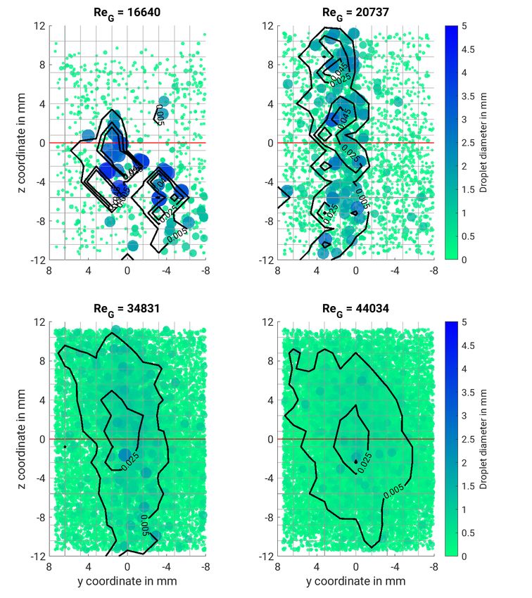
3.4. Droplet Spreading
This last section covers the deviation of the disintegrated droplets. Therefore, the lo-
cation of the droplets at position B is visualized. Figure 8 shows this visualization for
the same experimental cases, discussed above. Every droplet that is counted position B is
shown as a colored dot. The location is according to the measured value in the experiment.
The equivalent diameter of the droplet is visualized with the color and the size of the dot.
The position of the trailing edge accords to z = 0 and the rivulet is placed at y = 0, which
matches the center of the evaluation area. The first observation comparing the plots is
again the number of droplets and their spatial distribution. Although the small droplets at
ReG = 16,640 are spread widely across the whole area, their number is too small to cover
it completely. This is in contrast to the cases with ReG = 34,831 and ReG = 44,034, where
the whole area is covered with droplets. However, this mainly arises from the large number
of small droplets. Furthermore, it can be seen that the deviation strongly depends on
the droplet diameter. Large droplets show less deviation compared to small droplets.Aerospace 2021, 8, 91 12 of 15
Figure 8. Locations of droplets traveling through area at position B for four selected ReG numbers. Traced droplets are
marked with colored dots. Black contour lines show the normalized cumulated volume of droplets traveling through
predefined equal sized square patches (shown with grey grid lines). Trailing edge position is visualized with the red line.
This arises from the fact that the small droplets with the large deviations are mainly
ejected within the bag breakup regime. At the instance of bag breakup, the thin film
of the bag ruptures and small droplets are ejected radially into the air flow with a highAerospace 2021, 8, 91 13 of 15
velocity. This ejection velocity distributes them over the whole area. Larger droplets
don’t experience this strong acceleration and are therefore not distributed in the same
amount. At ReG = 16,640, most large droplets are located at z ≤ 0 mm, which is below
the trailing edge. This is due to gravity. At ReG = 20,737, the flapping of the ligament in
the xz-plane at asymmetric Rayleigh breakup also accelerates the larger droplets in this
plane and causes the visible deviation. To further compare the distribution of the droplets
quantitatively, the area has been divided into equally sized squares. These are indicated
in the plot with the grey grid lines. Within each square, the volume of all corresponding
droplets has been cumulated (Vsq ) and normalized by the total volume of all droplets
(Vtotal ). The contour lines represent these normalized values (Vsq /Vtotal ). From the contour
lines, it can be derived that, with increasing ReG number, the distribution of the droplet
volume across the area at position B gets more continuous. This qualitative statement
from optical observation of the contour plots can be confirmed quantitatively—on one
hand by the maximum value of Vsq /Vtotal and on the other hand by the area that shows
a value of Vsq /Vtotal ≥ 0.005. The calculated values are given in Table 2. It can be seen
that, for higher ReG numbers, the maximum value of Vsq /Vtotal decreases and the area
where Vsq /Vtotal ≥ 0.05 increases at the same time. Both indicates that the distribution
of the droplet volume is more continuous. The contour also shows how the transition from
a spotty to a continuous distribution happens. First, the distribution is spreading in the
z-direction. This is due to the up and downward flapping of the ligament in the asymmetric
Rayleigh breakup. As soon as bag breakup becomes more dominant, the radial spreading
of the droplets prevails and the distribution is also widened in the y-direction.
Table 2. Comparison of the cumulated and normalized droplet volume Vsq /Vtotal at position B.
ReG max(Vsq /Vtotal ) Vsq /Vtotal > 0.05
16, 640 0.182 13.3%
20, 737 0.082 24.0%
34, 831 0.042 37.3%
44, 034 0.047 39.3%
4. Conclusions
The performed experiments extend the database shown in [2]. The integral findings,
concerning the mean droplet diameter after disintegration and also the breakup regimes,
are in good accordance with [2]. The additional detailed evaluation of the experiments
gives the opportunity to model the disintegration process in a more complex manner. In
the following, the key findings will be summarized. The rivulet width at the trailing edge
is nearly constant for all examined ReG with a value of 2.7 mm and a standard deviation
S = 0.9 mm. The height is decreasing monotonously from 1.9 mm at ReG = 12,930
to a minimal value of 0.16 mm at ReG = 45,620. The maximum ligament length measured
from the trailing edge first increases until it reaches a maximum at ReG = 18,999 with
Llig = 7.81 mm. At higher ReG , bag break up occurs more often and the mean liga-
ment length decreases. Disintegration period and volume are strongly coupled and show
a monotonous asymptotic decrease with ReG towards the minimum disintegration pe-
riod of 0.006 s and disintegration volume of 1.3 mm3 . The observation of the resulting
disintegrated spray shows a change of the diameter distribution from a bimodal to a log-
normal distribution with the onset of bag breakup. Additionally, the mean diameter is
asymptotically decreasing to a minimum value of D10 = 0.19 mm. Droplet spreading
lateral to the air flow is strongly coupled to the breakup regime. At the symmetrical
Rayleigh breakup regime, mainly the central region behind the trailing edge will be hit.
At the asymmetrical Rayleigh breakup regime, the droplets spread vertically. With the on-
set of bag breakup, the droplets are spread both vertically and horizontally. Additionally,
the homogenity of the lateral distribution is increasing with ReG . These findings will help
to improve simulations of cases where trailing edge disintegration occurs. The futureAerospace 2021, 8, 91 14 of 15
scope will be to further extend the database to cover a larger range of ambient conditions.
Particularly interesting will be the dependence on the contact angle and the liquid mass
flow rate. In addition, the investigation of higher air flow velocities is considered to see if
another breakup regime can be seen, as for jet breakup. With this database, the existing
models shall be extended to cope with the above-mentioned requirements.
Author Contributions: Conceptualization, A.S. and B.W.; methodology, A.S.; software, A.S.; valida-
tion, A.S.; formal analysis, A.S.; investigation, A.S.; resources, B.W.; data curation, A.S.; writing—
original draft preparation, A.S. and B.W.; writing—review and editing, A.S. and B.W.; visualization,
A.S.; supervision, B.W.; project administration, B.W.; funding acquisition, B.W. Both authors have
read and agreed to the published version of the manuscript.
Funding: This research was funded by German Research Foundation (DFG) grant number
WE2549/36-1. The authors kindly acknowledge the financial funding by DFG.
Institutional Review Board Statement: Not applicable.
Informed Consent Statement: Not applicable.
Data Availability Statement: The data presented in this study are available on request from the
corresponding author.
Conflicts of Interest: The authors declare no conflict of interest.
Abbreviations
The following abbreviations are used in this manuscript:
α Incidence angle [◦ ]
CDF Cumulative distribution function
D Droplet diameter [m]
D10 Mean droplet diameter [m]
Din Needle inner diameter [m]
Din Needle outer diameter [m]
f Focal length [m]
fps Frames per second [1/s]
K Splashing threshold [-]
L Plate length
Llig Ligament length [m]
N Total number
PMMA Polymethylmethacrylat (Acrylic glass)
ReG Reynolds number of air flow [-]
ρD Liquid density [kg/m3 ]
ρG Air density [kg/m3 ]
σD Liquid–gas surface tension [N/m]
S Standard deviation
θ app Apparent contact angle [◦ ]
tp Plate thickness
uD Droplet velocity [m/s]
uG Gas velocity [m/s]
Vsq Cumulated volume in grid square [m3 ]
Vtotal Total droplet volume at position B [m3 ]
We Weber number [-]
xi Value at specific data point
x Mean value of x
References
1. Neupert, N. Experimentelle Untersuchung einer tropfenbeladenen Strömung in einer Ebenen Verdichterkaskade. Ph.D. Thesis,
Helmut-Schmidt-University, Hamburg, Germany, 2017.
2. Gomaa, H. Modeling of Liquid Dynamics in Spray Laden Compressor Flows. Ph.D. Thesis, University of Stuttgart, Stuttgart,
Germany, 31 October 2014.Aerospace 2021, 8, 91 15 of 15
3. Pilch, M.; Erdman, C.A. Use of breakup time data and velocity history data to predict the maximum size of stable fragments for
acceleration-induced breakup of a liquid drop. Int. J. Multiphase Flow 1987, 13, 741–757. [CrossRef]
4. Chou, W.-H.; Faeth, G.M. Temporal properties of secondary drop breakup in the bag breakup regime. Int. J. Multiph. Flow 1998, 24, 889–912.
[CrossRef]
5. Seck, A.; Geist, S.; Harbeck, J.; Weigand, B.; Joos, F. Evaporation Modeling of Water Droplets in a Transonic Compressor Cascade
Under Fogging Conditions. Int. J. Turbomach. Propuls. Power 2020, 5, 5.
6. Mundo, C.; Sommerfeld, M.; Tropea, C. On the modeling of liquid sprays impinging on surfaces. At. Sprays 1998, 8, 625–652.
[CrossRef]
7. Cossali, G.E.; Marengo, M.; Santini, M. Impact of single and multiple drop array on a liquid film. In Proceedings of the 19th
Annual Meeting of ILASS, Nottingham, UK, 6–8 September 2004.
8. Gomaa, H.; Stotz, I.; Sievers, M.; Lamanna, G.; Weigand, B. Preliminary investigation on diesel droplet impact on oil wallfilms in
diesel Engines. In Proceedings of the 24th European Conference on Liquid Atomization and Spray Systems, Estoril, Portugal,
5–7 September 2011.
9. Samenfink, W.; Elsäßer, A.; Dullenkopf, K.; Wittig, S. Droplet interaction with shear-driven liquid films: Analysis of deposition
and secondary droplet characteristics. Int. J. Heat Fluid Flow 1999, 20, 462–469. [CrossRef]
10. Feldmann, J. Aerodynamically Driven Surface-Bound Liquid Flows: Characterization and Modeling of Wetting Patterns.
Ph.D. Thesis, Technical University of Darmstadt, Darmstadt, Germany, 23 June 2020.
11. Lefebvre, A. Atomization and Sprays, 1st ed.; Hemisphere Pub. Corp.: New York, NY, USA, 1989.
12. Crowe, C.T. Multiphase Flow Handbook, 1st ed.; CRC Press: Boca Raton, FL, USA, 2005.
13. Dumouchel, C. On the experimental investigation on primary atomization of liquid streams. Exp. Fluids 2008, 45, 371–422.
[CrossRef]
14. Gepperth, S.; Koch, R.; Bauer, H.-J. Analysis and Comparison of Primary Droplet Characteristics in the Near Field of a Prefilming
Airblast Atomizer. In Proceedings of the ASME Turbo Expo 2013: Turbine Technical Conference and Exposition, Volume 1A:
Combustion, Fuels and Emissions, San Antonio, TX, USA, 3–7 June 2013.
15. Chaussonnet, G.; Gepperth, S.; Holz, S.; Koch, R.; Bauer, H.-J. Influence of the ambient pressure on the liquid accumulation
and on the primary spray in prefilming airblast atomization. Int. J. Multiph. Flow 2020, 125, 103229. [CrossRef]
16. Kim, W. Study of Liquid Films, Fingers, and Droplet Motion for Steam Turbine Blading Erosion Problem. Ph.D. Thesis,
University of Michigan, Ann Arbor, MI, USA, 1978.
17. Hammitt, F.G.; Krzeczkowski, S.; Krzyżanowski, J. Liquid film and droplet stability consideration as applied to wet steam flow.
Forschung im Ingenieurwesen A 1981, 47, 1–14. [CrossRef]
18. Javed, B.; Watanabe, T.; Himeno, T.; Uzawa, S. Effect of trailing edge size on the droplets size distribution downstream of the blade.
J. Therm. Sci. Technol. 2017, 12, JTST0031. [CrossRef]
19. Javed, B.; Watanabe, T.; Himeno, T.; Uzawa, S. Experimental investigation of droplets characteristics after the trailing edge at
different angle of attack. Int. J. Gas Turbine Propuls. Power Syst. 2017, 9, 32–42. [CrossRef]
20. Farago, N.; Chigier, Z. Morphological classification of disintegration of round liquid jets in a coaxial air stream. At. Sprays 1992, 2, 137–153.
21. Cengel, Y.; Cimbala, J. Fluid Mechanics: Fundamentals and Applications, 1st ed.; McGraw-Hill: Boston, MA, USA, 2006; pp. 325–326.You can also read