Unequal Mortality during the Spanish Flu - LSE Research Online

Economic History Working Papers No: 325

 Unequal Mortality during
 the Spanish Flu

 Sergi Basco, Universitat de Barcelona;
 Jordi Domènech, Carlos III de Madrid;
 and Joan R. Rosés, LSE

 February 2021

 Economic History Department, London School of Economics and Political Science,
 Houghton Street, London, WC2A 2AE, London, UK. T: +44 (0) 20 7955 7084.

Unequal Mortality During the Spanish Flu
 Sergi Basco, Jordi Domènech and Joan R. Rosés•

Keywords: Pandemics, Health Inequality, Socio-Economic Mortality Differences, Urban Penalty.
JEL codes: N34, J1, I14

 Abstract
 The outburst of deaths and cases of Covid-19 around the world has renewed the
 interest to understand the mortality effects of pandemics across regions, occupations,
 age and gender. The Spanish Flu is the closest pandemic to Covid-19. Mortality rates
 in Spain were among the largest in today’s developed countries. Our research
 documents a substantial heterogeneity on mortality rates across occupations. The
 highest mortality was on low-income workers. We also record a rural mortality penalty
 that reversed the historical urban penalty temporally. The higher capacity of certain
 social groups to isolate themselves from social contact could explain these mortality
 differentials. However, adjusting mortality evidence by these two factors, there were
 still large mortality inter-provincial differences for the same occupation and location,
 suggesting the existence of a regional component in rates of flu contagion possibly
 related to climatic differences.

1. Introduction
Mortality rates during modern pandemics are unequal (Bambra et al, 2020; Chen and Krieger, 2021;
Feigenbaum et al. 2019; Turner-Musa at al., 2020). Pandemic deaths hit countries, regions, sexes,
ages and social classes with a surprisingly large variation in intensity. The timing of the arrival of
the pandemic and the precautionary measures can explain a considerable amount of the geographic
variation in mortality (Markel et al., 2007). Some intrinsic characteristics of the affected locations
like population density and climate can also account for these geographical patterns (Mamelund,
2011; Clay at al. 2018, 2019). Genetic differences or previous immunization to the pandemic shape
sex and age mortality differentials (Noymer, & Garenne, 2000). However, social group mortality
differences are not easy to explain (Mamelund, 2017). On the one hand, there is co-morbidity
caused by living conditions (poor housing, nutrition and sanitation) and social-related illness
(Brown and Ravaillon, 2020). On the other hand, poor people could not avoid social contact

•
 Correspondence: Sergi Basco: Universitat de Barcelona (sergi.basco@ub.edu); Jordi Domènech: Carlos III de
Madrid (jdomenec@clio.uc3m.es); Joan Rosés: London School of Economics and CEPR (j.r.roses@lse.ac.uk).

 1

during pandemic outbursts and, hence, suffer a large proportion of infections (Jay at al., 2020).
Furthermore, some jobs have a higher infection, and hence mortality risks, than others.

The main contribution of this paper is to uncover the substantial unequal mortality differentials
during the 1918-flu pandemic. Specifically, we consider deviations from historical mortality trends
across age, sex, space (provinces and rural versus urban) and occupational groups in Spain. There
are several reasons why this country is an excellent natural experiment of the dramatic
consequences of this pandemic without pharmacological control. Mortality rates were very high,
among the highest in the developed world, and experimented large spatial differences. The
population was fully representative of all age groups since the country was neutral during World
War I meaning young male adults were not overseas fighting. Instead of what happened in
belligerent countries, where information on the pandemic was censored by the military, Spain's
population were aware of the spread of the illness and authorities publicised and implemented
several measures to fight the pandemic. Finally, the Historical Database of INE (Spanish National
Statistical Office) provides disaggregated data on the localisation, sex, age, and occupation of the
deceased.

For the flu pandemic of 1918, the broad regional and socio-economic differences in mortality are
not fully understood (Herring and Korol, 2012; Mamelund, 2006 and 2018; Økland and
Mamelund, 2019; Sydenstricker, 1931; Tuckel et al., 2006; Vaughan, 1920; and Wilson et al. 2014).
In most cases, the sparse evidence came from local studies assembling flu-related mortality data at
low levels of disaggregation and analysing their correlation with a series of socio-economic
indicators at the same level of disaggregation. The typical socio-economic indicators considered
are population density, illiteracy rates, homeownership rates, number of rooms per household and
unemployment (Grantz et al., 2016; Mamelund, 2006, 2018; Vaughn 1920). Most of these studies
point to a strong link between socio-economic indicators and flu-related mortality. Less developed
regions tend to have higher mortality rates, albeit the causal link and the specific channel between
these socio-economic indicators and mortality differentials are hard to establish (Chowell and
Viboud, 2019. Moreover, localised studies can only explain a small part of the overall regional
variation in mortality levels (Pearl, 1921; Chowell, Erkoreka et al., 2014).

According to our research, the main features of Spain’s flu mortality are the following. First, the
mortality differences among different professions are impressive (excess mortality ranged from
102% for miners to 19% for rentiers). Second, these differences are also substantial when we

 2

aggregate occupations for socio-economic groups. The high-income group (liberal professions and
rentiers) had an average excess mortality rate of 29% compared to 69% in the low-income group
(agriculture and mining) and 62% in the mid-income group (industry, trade and transport). These
evidence points in the direction that these mortality differentials were related to the higher capacity
of certain social groups to isolate themselves from social contact. Third, we also document a female
penalty. For example, the excess mortality rate during pandemic peak (October 1918) was 374 per
cent for females and 321 per cent for males. Fourth, another defining characteristic of the Spanish
Flu is an inverse U-shape in excess mortality rate. The peak was in people aged between 25 and
29. Fifth, the paper undercovers an urban premium with rural mortality rates exceeding urban ones
in each occupation during 1918-flu. However, despite this flu-related rural penalty, the overall
urban penalty did not disappear, even during 1918 (Reher, 2001). Sixth, using shift-share analysis,
we point out that the provincial component explains most of the spatial variation in mortality rates.
We also demonstrate that the mortality differentials of certain provinces had a remarkable
geographic element (latitude), which may be related to weather differences. Finally, we document
a negative correlation of development levels, measured with population density, with excess
mortality in occupations in the low-income group.

The rest of the paper is organized as follows. Section 2 reviews the chronology of the flu in Spain
and the different non-pharmacological measures taken by public authorities. The following section
considers mortality differentials between sexes and among different age groups. Section 4 discusses
heterogeneous excess death rates across occupations and rural/urban locations. The subsequent
section decomposes them with a shift-share method. The last section concludes.

2. The Spanish Flu in Spain: Chronology and Public Measures
This section will review the basic information on the development of the Spanish flu in Spain.
Therefore, we will consider the chronology of the pandemic, how the news on the pandemic
spread, and what measures were taken to respond to its development.

A substantial Spanish Flu literature argues the existence of three waves in this pandemic: a first
wave during the summer of 1918; a second one in the fall of 1918 and a third, milder one, during
the Winter 1918/19 (See, for example, Chowell, Erkoreka, et al. 2014, for Spain; Pearce et al.,
2010, for England and Wales; and Taubenberger and Morens, 2006, for a summary review). To
review if this chronology applies to Spain, we will measure the Monthly Excess Death (MEDt):

 3

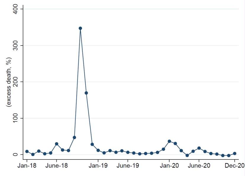
 ℎ 1918 
 = 100 ∗ [ − 1], (1)
 ℎ −1918 

where t is the Month when average death pre-1918 is calculated as average deaths between 1911
and 1917. Note that this measure of excess mortality rate accounts for potential seasonal mortality
effects and controls for age differentials of mortality.

An alternative approach is to calculate mortality rates using the official registrar declaration of the
cause of death. These data are available for Spain and have been used previously by Chowell,
Erkoreka et al. (2014). However, this information has problems. In the early 20th century, the
cause of death was recognized by the symptoms since no test of flu-infection existed. Therefore,
it is likely that doctors were underreporting flu-related mortality at the beginning of the pandemic
and exaggerating its impact during its later phases. The disparate behaviour of the different local
doctors and registrars influenced the reporting of the mortality cause. As a comparative
assessment, the Spanish registrars identified in 1918 a total of 147,114 flu deaths and 117,778
deaths caused by other respiratory problems, which some authors directly attributed to flu. Instead,
with our method, the total figure of excess deaths is 245,406. For the record, the Spanish registrars
detected 7,749 flu deaths and 44,463 caused by other respiratory problems in 1917.

Figure 1. Evolution of Monthly Excess Mortality

Source: Historical Database of the Spanish National Institute of Statistics (INE).

 4

Figure 1 represents the overall series of monthly excess mortality. Our data partly confirms the
presence of three waves albeit the second is several times bigger than the other two.1 We can
observe a small peak in June of 1918 (excess mortality was around 30 per cent), which, maybe,
could be labelled as the first wave. The second wave started in September, reaching a peak in
October and bottoming up in December. Quantitatively, the peak in excess mortality in October
is shocking. The number of deaths more than quadrupled those commonly observed in October
(to be precise, the increase was 347 per cent). Even though excess mortality in November was
significantly lower than in October, it still implies that the number of deaths more than double
those typical in November (169 per cent increase). There is no sight of the third wave in the winter
of 1918/19. Indeed, the only “wave” after October 1918, it is a spike in January of 1920, which
seems farfetched to consider it the third wave of the Spanish Flu. A plausible explanation for the
small significant third wave in Spain is that the fall wave was so intense and the exposure so
widespread that inhabitants gained immune protection (Barry et al., 2008; and Pierce et al., 2010).

Contrary to what happened in the belligerent countries, the Spanish press regularly informed on
the pandemic. To illustrate the evolution of the presence of the flu in the media, Figure 2 displays
the timeline of mentions to “epidemic” and “grippe” (the French word for flu typically used in
Spain) in the leading Barcelona newspaper, La Vanguardia, (hereafter LV).

1 Chowell, Erkoreka et al (2014) also claims the presence of three waves in the flu in Spain. However, the Spanish
evolution of the pandemic it is clearly different to the English and Wales’ one (figure 1 in Pierce et al., 2010), where
the three waves are clearly visible at first sight, with the peak in excess mortality in the third wave of around half the
second.

 5

Figure 2. Evolution of Flu-Related Mention in the News
 400
 370
 350

 300

 250 252

 200

 150

 100 112
 97 91
 83 75
 50 44 55
 42
 30 30 32 33 32 24 30 24
 12 20 11 4 21 16
 7
 25 15 16 16 23 20 12 22 26 26
 0 0

Notes: Times the word “epidemic” and “grippe” are mentioned in LV, from January 1918 to December 1920.
Source: Underlining data has been obtained from LV’s online newspaper library
https://www.lavanguardia.com/hemeroteca.

As we can see, there was a mild increase in newspaper hits for these two words in April, which
peaked in June 1918 at around seven times the value in January. Although the disease had diffused
widely among military cadets and the army cancelled their yearly parades, the mood in May 1918
was optimistic.2 On 25th May 1918, the famous doctor Gregorio Marañon noted that all the
pandemic cases had a favourable evolution in Madrid and it was a “mild” flu epidemic.3 However,
newspapers informed that many workers were ill in Madrid (tram drivers, doctors, postal office
and health inspectors) and Granada (textile workers).4

The number of hits declines during the summer coming back to the start of the year figures. The
series started to grow exponentially in September, reaching in October a value 30 times larger than
the first months of the year. After the peak in October, the series slightly declined in November:
the number of hits was still 20 times larger than in January. The number of hits continued to fall
in the Winter. During the first months of 1919, the number of hits was around eight times larger
than one year before but substantially lower than the peak in October 1918. After March 1919, the
presence of flu-related words declined again, and it seems to stabilize to a value slightly larger than
the start of the sample. In sum, the pandemic news and its mortality followed a similar pattern.

2 El Restaurador, 22nd May 1918: 3; Diario de Cádiz, 23rd May 1918: 3.
3 LV, 25th May 1918, p. 8).
4 La Correspondencia de España, 24th May 1918, p. 4. In Granada, for example, many women employed in the textile

sector had fallen sick, in some cases forcing some establishments to close completely as all personnel was sick (LV,
2nd June 1918, p. 14).

 6

The Spanish newspapers also report, with substantial detail, the measures taken by the authorities
to control the pandemic. In each province, the prefect (the highest government political authority)
and the health commission (“Junta Provincial Sanitaria”) could officially declare the existence of a
pandemic and implement different measures.5 On broad terms, the contemporary scientific
understanding of contagion channel was reasonably accurate. The main official recommendations
were avoiding crowded and poorly ventilated spaces, multitudes and washing hands often. The
authorities cancelled many festivals and local fairs and holidays.6 Primary and secondary schools,
seminaries, high and technical schools and universities did not re-open after the summer harvests
and festivities.7 Dance and music halls and theatres were closed. The government also cancelled
the Military replacements to limit the contagion by infected conscripts to other soldiers.8 In
prisons, sick prisoners were isolated and given medical treatment. However, there is scarce
evidence of the wearing of masks, and no evidence of strict lockdowns and the closing of
establishments, workshops and stores (except when all their workers were sick) enforced by
authorities. Similarly, harvests took place since we cannot observe an agricultural production
decrease (Basco et al. 2021). All in all, these set of measures denote the existence of some prior,
accumulated knowledge of dealing with epidemics, especially in urban settings (Rodríguez-Ocaña,
1994).

3. Inequality in Mortality Among Sex and Age Groups
In this section, we will discuss the heterogeneity mortality across sex and age groups. Employing
the same methodology than Figure 1, Figure 3 considers monthly excess mortality. The same
pattern is apparent for both males and females. There was a large increase in excess death in
October, followed by a less secondary peak in November, and no other month with significant
death rates. However, another feature of Figure 3 is that excess mortality was higher for females.
In October 2018, the excess death rate was 321 per cent for males (Panel A) and 374 per cent for
females (Panel B). Overall, it was a female penalty: the total excess female mortality was 57 per
cent while the male one was only 51 per cent.

5 For example, in the province of Valladolid, LV, 2nd October 1918, p. 14.
6 LV, 29th September 1918, p. 17.
7 LV, 29th September 1918, p. 17; LV, 1st October 1918, p. 12.
8 LV, 19th September 1918, p. 15; LV, 1st October 1918, p. 12.

 7

Figure 3: Evolution of Monthly Excess Mortality (by gender)
a) Male

b) Female

 Source: See Figure 1.

Figure 4 reports the excess death rates by age group and gender (see Table 1A at the appendix for
the actual numbers). Excess death rates follow an inverse U-shape: they were lower for children
and older adults than young people. The age-group with the higher mortality rates was the age-

 8

group from 25 to 34 years old. This age-group has an excess death rate of above 200 per cent. In
contrast, people above 55 years old had an excess death rate of below 40 per cent. These findings
on relatively lower excess mortality for older adults are consistent with previous evidence on the
Spanish Flu (Schoenbaum, 1996; Luk et al. 2001). The literature has argued that it was likely that
older adults had already gone through other flu episodes and had acquired immunity to this flu
pandemic.

Figure 4: Excess Mortality Rate by Age Group

 Source: See Figure 1.

If we focus on the absolute number of excess deaths (rather than the excess rate), the pattern
changes. Figure 5, and Table 1A, reports the distribution of the number of excess deaths across
age groups. We now obtain a clear W-shape, with three identified peaks: (1) children aged between
1 and 4 years; (2) adults between 25 and 29 years old; and (3) elders with more than 60 years. 9
However, as we have seen in Figure 3, the second group was the only one in which excess death
rate increased dramatically in 1918. In other words, children and older adults had already higher
mortality before the pandemic and, thus, a large increase in the overall number of deaths resulted
in a relatively small increase in their excess death rates. Taubenberger and Morens (2006) argue
that Spanish Flu W-shape has not been documented for any other pandemic since excess deaths
in pandemics take a U-shape form.

9 Taubenberger and Morens (2006) obtained the same pattern for the United States.

 9

Figure 5: Excess Mortality by Age Group

Source: See Figure 1.

4. Heterogeneous Excess Death Across Occupations Considering Urban-Rural
 Locations.
This section reports the main results of the paper. We examine the potential heterogeneity of
excess mortality (following the equation 1) during the Spanish Flu across occupations and gender
separately by urban and rural locations. Furthermore, we also aggregate mortality in 3 different
income groups. The following table 1 reports the occupational mortality rates by gender and urban
and rural settings.

 10

Table 1: Excess Mortality by Occupation, income, location and sex in 1918 (per cent)
 Urban Rural Overall
 Male Female Total Male Female Total Male Female Total
 (1) (2) (3) (4) (5) (6) (7) (8) (9)
Panel A (occupations)
(i) Agriculture 51.98 43.81 51.49 73.15 50.86 69.13 72.41 50.79 68.59
(ii) Mining 58.67 58.67 105.82 105.82 101.80 101.80
(iii) Industry 39.05 31.04 38.48 68.44 52.48 67.32 60.94 46.93 59.95
(iv) Transport 53.42 53.21 90.43 90.48 81.44 81.43
(v) Trade 6.70 3.62 57.75 50.55 42.52 37.23
(vi) Armed forces & Police 95.06 95.06 104.69 104.69 99.72 99.72
(vii) Administration 12.02 12.45 50.74 50.55 36.61 36.65
(viii) Liberal Professions 34.54 26.75 32.77 59.56 41.83 55.94 51.14 36.29 48.00
(ix) Rentiers 16.95 -5.86 13.60 17.42 29.62 19.47 17.35 24.71 18.56
(x) Domestic Workers 25.98 54.00 53.87 65.05 78.87 78.84 49.65 73.51 73.45
(xi) No Occupation 47.37 62.99 47.48 62.95 104.73 65.64 57.47 102.42 59.49
(xii) Unknown/Non-
productive 32.83 26.04 29.95 42.01 43.11 42.51 40.04 39.81 39.94
Overall 38.57 41.55 40.01 54.69 61.51 58.05 51.77 57.63 54.49
Panel B (income
groups)
(a) Low-income 52.17 43.81 51.68 73.51 50.86 69.47 72.76 50.79 68.92
(b) Mid-income 38.74 24.95 37.93 71.59 45.54 69.97 63.18 40.48 61.79
(c) High-income 26.41 15.81 24.37 30.13 33.95 30.81 29.31 29.66 29.37
Overall 38.30 21.67 36.55 68.12 48.41 64.87 65.24 46.81 62.30

 Notes: Urban are deaths in the provincial capital while rural are deaths in the rest of the province. Spanish literature
 uses the same definition of the urban and rural population (Reher, 2001). The official statistics classified children as
 non-productive. There are very few women working in the transport, trade sector and administration; so, their data is
 not presented but considered for overall calculations. Agricultural and mining workers make the low-income group.
 Workers in industry, trade and transport make the mid-income. Liberal occupations and rentiers make the high-income
 one. We do not consider in Panel B domestic workers, armed forces & police, no occupation and unknown, and non-
 productive given uncertainty on their income levels.
 Source: See Figure 1.

 Looking at Panel A (column 9), we observe that the occupations for which excess mortality
 increased the most were workers in mining, armed forces & police, and transportation (with
 increased death rates above 80 per cent). These results seem consistent with the view that flu
 contagion was higher in occupations in which people were in close contact. Workers in the mineral
 sector had the additional disadvantage of working in places with poor ventilation, where it has
 been shown there is faster diffusion of the virus (Brundage and Shanks, 2008). Similarly, people
 employed the armed forces & polices, and transportation had to move across villages and,
 arguably, had high exposure to the flu. Also, the military personnel lived in barracks sleeping in
 communal dorms, which facilitated the spread of the flu. On the other side of the mortality
 spectrum, one can observe the lowest mortality rates among rentiers (only 18 per cent). It is

 11

plausible that rentiers were more aware of the dangers of the flu, were not forced to leave the
house to work, and kept social distancing.

Although the occupational differences were staggering, there are two potential sources of bias in
our analysis exacerbating the occupational mortality differentials. First, age is a concern since it is
likely that rentiers were older than other workers and we have shown in the previous section that
the group between 20 and 50 years was the group with the highest mortality. Second, geography
is another potential source of bias because mining was only present in some parts of the country.
However, the evidence presented in panel A provides strong evidence that the occupation affected
the probability of contagion and, thus, excess mortality.

A plausible interpretation of panel A is that workers in high-income occupations had the economic
means (savings) and knowledge to better shield against the pandemic. To give further support to
this interpretation, we classify occupations in three income groups: (a) low-income, (b) mid-income
and (c) high-income. Panel B reports excess mortality in 1918 for each of these groups. It becomes
apparent from the table that high-income occupations have substantially lower excess mortality.
Quantitatively, excess mortality in 1918 was 29 per cent higher than their historical average among
high-income workers. The increase in mortality was higher among low- and mid-income
occupations with 69 per cent and 62 per cent, respectively. Since in panel B, we are aggregating
occupations, the concerns on the biases introduce by age and geographically concentrated
mortality diminish.

The dataset contains information on the number of deaths by occupation decomposed between
males and females. We report these computations in Table 1, Panel A, columns 7 and 8. The goal
of this exercise is twofold. Firstly, we want to compare the influence of gender on our estimates
of excess mortality by occupation. In other words, we want to test if females had more mortality
performing the same job as males. Secondly, we use the excess mortality differentials by gender as
a robustness check of the result that high-income occupations had low excess mortality. It is
important to note that a relevant characteristic of Spanish labour markets in the 1910s was the
substantial segregation by gender: men were rare in the domestic sector while females were scarce,
or absent, in mining, transport, trade, armed forces & police, and administration (Nicolau, 2005).
Another problem was that census officials classified many female agricultural workers as no
occupation or domestic workers (Gil Ibáñez, 1978)

 12

We conclude from this exercise that higher female mortality was mainly due to a compositional
effect. On the one hand, mortality was higher in the two “female” occupations (domestic workers
and the group with no reported occupation). On the other hand, male mortality was higher in
occupations with the two sexes (agricultural, industry and liberal professions). The only exception
is rentiers, for which female mortality was higher than male mortality. Similarly, in Panel B, where
we group occupations in three large income groups, we observe a very similar mortality pattern
for male and female, which is consistent with the aggregate numbers discussed above. Females
and males working in high-income occupations had substantially smaller excess mortality than
those working in low- and mid-income occupations. The numbers for high-income occupations
are almost the same for males and females. Excess mortality is high for males in low- and mid-
income industries, which is partly due to the overrepresentation of males in some occupations.

We now turn the descriptive analysis of the heterogeneity between urban and rural locations (Table
1, columns 1 to 6). The consensus in the literature is that there was an urban penalty in mortality
during industrialization. Urban mortality was higher until the discovery of pharmaceutical
measures and large investments in urban sanitation (e.g., Cain and Hong, 2009; Evans, 2006, and
Haines, 2001). In Spain, the urban penalty was present, at least, until the Spanish Civil War but it
was lower than in other European countries (Reher, 2001; Ramiro and Sanz 1999; García Gómez,
2016). This urban penalty was higher among working-classes and was clearly observable in heights
of conscripts (Martínez-Carrión and Moreno-Lázaro, 2006). The main causes of it are purely
structural: poor sanitation, inadequate housing, food quality and harsh working conditions
(Escudero and Nicolau, 2014). In pandemics, overcrowding in cities should lead to more contagion
and thus higher mortality (Haines, 2001). However, people in the cities may have better
information on the evolution and dangers of influenza, they might take more stringent social
distance measures, this reducing contagion and mortality. Furthermore, income and wages were
higher in Spanish cities than in the countryside (Rosés and Sánchez-Alonso 2004) and, hence,
urban workers could have more savings to keep the social distance.

When looking at the urban-rural mortality differentials, our results are very consistent: the rural
mortality premium is higher across all different occupations for male and female deaths. For
example, among workers in the industry, rural locations had 75 per cent higher excess mortality
rate than cities. For the rest of the occupations, the rural excess mortality in male and female was
between 40 and 70 per cent higher. Given that this urban mortality advantage was not due to
structural health factors, it is likely that social distancing measures played a substantial role in these

 13

death differentials. Furthermore, these results also cast doubts about the hypothesis that previous
sanitary or health conditions were decisive for mortality rates.

Next, we turn our income-group classification in Panel B. As expected, the differences in this table
are lower than the counterparts in Panel A. However, we observe substantial heterogeneity: High-
income occupations were the ones for with the smaller urban mortality advantage in the cities.
One potential explanation is that high-income occupations in rural and urban areas had enough
information and resources to remain isolated and shielded against the flu. Interestingly, the largest
urban advantage is in mid-income occupations (industry, trade and transport), although there is
very limited evidence of factories closures.

5. Decomposing Flu Mortality
In this section, we will employ a shift-share analysis and a basic regression framework to
disentangle some factors behind the spatial differences in Flu mortality across Spanish provinces.
Specifically, we decompose the change in the number of deaths per inhabitant in province c and
occupation o as,

 ∆ ℎ , = , + , + , + , , (2)

where,
 , = ℎ , , −1918 ∗ ∆ ℎ , 
 , = ℎ , , −1918 ∗ (∆ ℎ , − ∆ ℎ , )
 , = ℎ , , −1918 ∗ (∆ ℎ , − ∆ ℎ , )

Note that the Aggregate Component represents the increase in the number of deaths arising from the
aggregate national effect of the flu in Spain, which is akin to a year fixed effect. The Rural Component
represents the increase in the number of deaths since there were a rural penalty and controls for
rural occupations. As we have seen, for the same occupation, mortality was higher for workers in
that occupation outside the capital or main city. The Urban Component is the analogous of the rural
component. Finally, the Province Component is the residual component and represents the specific
mortality of the province in a particular occupation. Analytically, the Province Component is:

 14

 ℎ , , −1918 ∗ (∆ ℎ , − ∆ ℎ , ) +
 + ℎ , , −1918 ∗ (∆ ℎ , − ∆ ℎ , ) +
 + ℎ , , −1918 ∗ (∆ ℎ , − ∆ ℎ , ).

Since we are interested in total excess mortality, note that the third term cancels out. That is, when
o=total, the third term is zero.

Table 2A at the appendix reports the numbers. We report for each province c, where =
∑ , for = { , , }. Note that in this exercise we control for
the size of the population. The most important component to explain the increase in the number
of deaths in each province is the Aggregate Component. Specifically, it explains about 95 per cent
of the variation in provincial deaths.

The following figure 6 reports the importance of all components except the aggregate component
for the relative number of deaths in each province.

Figure 6: Three Shift-Share Components by 1000 people
 Alava
 Albacete
 Alicante
 Almeria
 Avila
 Badajoz
 Baleares
 Barcelona
 Burgos
 Caceres
 Cadiz
 Castellon
Ciudad Real
 Cordoba
 Coruna
 Cuenca
 Girona
 Granada
Guadalajara
 Guipuzcoa
 Huelva
 Huesca
 Jaen
 Leon
 Lleida
 Logrono
 Lugo
 Madrid
 Malaga
 Murcia
 Navarra
 Orense
 Oviedo
 Palencia
Pontevedra
 Salamanca
 Santander
 Segovia
 Sevilla
 Soria
 Tarragona
 Teruel
 Toledo
 Valencia
 Valladolid
 Vizcaya
 Zamora
 Zaragoza
 -10 -8 -6 -4 -2 0 2 4 6 8 10 12
 PROVINCE RURAL URBAN

Notes: See the text for the definition of the aggregate, industry and province components.
Source: Appendix Table 2.A.

 15

Several results stand out from this figure. The urban (grey bar) and rural (orange bar) components
pull in opposite directions, as predicted. The urban component reduced mortality, so more
urbanized provinces had less flu-related mortality, while the contrary holds for the rural
component: more rural provinces experienced greater flu-related mortality. However, the most
relevant component in the graph is the province component (blue bar). There are substantial
differences across provinces: its average value is 0.48 and the standard deviation is 396 per cent.

Given its essential importance in explaining differences in mortality rates across provinces, it is
worth exploring the province component further. The five provinces with the lowest (negative)
province component were Cádiz (-6.38), Málaga (-6.18), Sevilla (-6.11), Cáceres (-5.29), and Girona
(-4.71). On the other extreme, the five provinces with highest province component were Almería
(9.11), Zamora (8.19), León (7.42), Burgos (6.85) and Orense (6.65). Interestingly, provinces in
each group are mostly co-located. The following map (Figure 7) confirms the spatial nature of the
province component.

Figure 7: Province shift-share component (by 1000 people)

Notes: See Figure 6.
Source: Appendix Table 2.A

 16

This map confirms the geographical component of flu mortality: most of the worst affected
provinces were in the Northwest of Spain and the least affected in the Guadalquivir Valley and
South Castile. However, we can also observe other salient peculiarities: the relatively high impact
in the mining-intensive provinces (Almeria, Huelva and Biscay) and the lesser impact of the
pandemic in the most urbanized provinces (Madrid, Barcelona, Valencia and Seville).

To explore further the previous results, we perform a regression analysis of the province
idiosyncratic component separately for each income group. In other words, we investigate if each
income group has different behaviour and if the geographical component is robust. Specifically,
we consider OLS specifications of the following form,

 _ = + + , (3)

where _ is the province component of excess mortality, weighted by population in order to
avoid Heterokedasticity, and are the provincial characteristics. Finally, note that since we focus
on the province components, equation (3) is akin to performing a regression with industry and
time fixed effects. That is, we removed the variation driven by sectoral composition and the
aggregate effect.

Table 2: Determinants of the Province effect

 Low-income Mid-income High-income Total Adults
 (1) (2) (3) (4) (5)
Density -14.46*** 1.32 -0.03 -6.67 -11.49
 (4.26) (0.96) (0.74) (13.56) (7.41)
Longitude -0.47 -0.17 -0.09 -0.61 0.45
 (0.71) (0.16) (0.07) (2.02) (1.36)
Latitude 1.27* 0.15 0.13 7.69*** 3.97**
 (0.65) (0.13) (0.097) (2.66) (1.54)
No Obs. 48 48 48 48 48
R2 0.23 0.14 0.05 0.21 0.16

Notes: * p < 0.10, ** p < 0.05, *** p < 0.01.
Sources: Appendix Table 2.A.

Table 2 reports the coefficients of running equation (3), with robust standard errors in parenthesis,
when considering different occupational groups. Our independent variables are the density of the

 17

province in 1910, longitude and latitude.10 Column 1 considers excess mortality in the low-income
group. For this group, the coefficient of population density is negative and statistically significant.
This result implies that provinces with higher population density (a proxy of urbanization and
economic development) had less excess mortality in low-income occupations (agricultural and
mining workers). Quantitatively, the effect is important: a one standard deviation increase in
population density reduces the province component of low-income mortality by 50 per cent
(-14.61*0.034). In this case, another relevant variable is the latitude, albeit significant only at 10 per
cent.

We consider medium and high-income occupations in column 2 and 3, respectively. In these two
cases, none of the variables is significantly different from zero. One interpretation is that these
individuals employed in mid- and high-income occupational groups were shielded from the flu in
all provinces. Finally, when we consider overall excess mortality (column 4), we notice that only
the latitude coefficient is statistically significant and quantitatively important: a one standard
deviation in latitude reduced the province component of mortality in 1918 by 170 per cent (-
7.69*0.22). Thus, it seems that being in the South helped substantially to prevent an increase in
mortality during 1918, as confirmed previously by figure 7. A growing literature has highlighted
latitudinal and climatic variations in contemporary influenza epidemics and pandemics (e.g.,
Alonso et al. 2007; Bloom-Feshbach at al. 2013; Tamerius et al. 2013), and in the severity and
timing of the 1918-flu (Chowell, Erkoreka, et al. 2014; Chowell, Simonsen at al. 2014; Reyes et al.
2018).

6. Concluding Remarks
In this paper, we have documented the unequal effects of pandemics on mortality across different
dimensions. This question has received renewed interest after the outburst of Covid-19. We have
focused on the mortality consequences of the Spanish Flu in Spain (1918). By using a historical
episode, we have the advantage of examining a fully completed event. Also, Spain in 1918
resembles a current developing economy in which social distancing is difficult due to budget
constraints, which can help us to extrapolate it to the effects of Covid-19 to developing countries.

10We also run several robustness regressions including more variables (GDP per capita, inequality and Population)
and with Conley Spatial Standard Errors. The results confirm our views of table 2 but Latitude lost significance. These
calculations are available in the appendix, Table 3A.

 18

Our main result is that the excess mortality rate in 1918 substantially varied across occupations
from 102% for miner workers to just 19% for rentiers. One interpretation is that whereas rentiers,
and other workers with middle incomes and high ones, were able to isolate, less affluent workers
were not and continued with their normal daily activities. Perhaps surprisingly, we also document
an urban premium. Indeed, excess mortality was lower in the capitals of provinces for all
occupations. When analysing the determinants of excess mortality, we find that latitude is the main
explanatory variable for overall mortality. For low-income workers, population density has a
negative correlation with mortality. These results are consistent with the presence of this urban
premium.

What is the implication of this study for the current Covid-19 crisis? Access to information, health
measures and medical knowledge have dramatically improved compared to 1918. Furthermore,
the 1918 flu has a substantially different age-related component since the most affected were the
young adults. However, a plausible interpretation of our findings is that awareness of the pandemic
and isolation seem critical to reduce mortality. Therefore, fully informed individuals who could
avoid working outside the home experienced much lower mortality rates. This result strongly
resonates with the current socio-economic differences in Covid-related mortality.

 19

References
Alonso, W. J., Viboud, C., Simonsen, L., Hirano, E. W., Daufenbach, L. Z., & Miller, M. A. (2007).
 Seasonality of influenza in Brazil: a traveling wave from the Amazon to the
 subtropics. American journal of epidemiology, 165(12), 1434-1442.
Bambra, C., Riordan, R., Ford, J., & Matthews, F. (2020). The COVID-19 pandemic and health
 inequalities. Journal of Epidemiology & Community Health, 74(11), 964-968.
Basco, S., J. Domènech, & Rosés, J.R. (2021): The Redistributive Effects of Pandemics: Evidence
 from the Spanish Flu, World Development, 141.
Barry J., Viboud, C., & Simonsen, L. (2008): Cross-protection between successive waves of the
 1918–1919 influenza pandemic: epidemiological evidence from US Army camps and from
 Britain. Journal of Infectious Diseases, 198, 1427–1434.
Bloom-Feshbach, K., Alonso, W. J., Charu, V., Tamerius, J., Simonsen, L., Miller, M. A., &
 Viboud, C. (2013). Latitudinal variations in seasonal activity of influenza and respiratory
 syncytial virus (RSV): a global comparative review. PloS one, 8(2), e54445.
Brown, C.S. & Ravallion, M. (2020). Inequality and the Coronavirus: Socioeconomic Covariates of Behavioral
 Responses and Viral Outcomes Across US Counties (NBER Working Papers 27549). Cambridge
 Ma national Bureau of Economic Research.
Brundage, J. F., & Shanks, G. D. (2008). Deaths from bacterial pneumonia during 1918–19
 influenza pandemic. Emerging infectious diseases, 14(8), 1193.
Cain, L., & Hong, S. C. (2009). Survival in 19th century cities: The larger the city, the smaller your
 chances. Explorations in Economic History, 46(4), 450-463.
Chen, J. T., & Krieger, N. (2021). Revealing the unequal burden of COVID-19 by income,
 race/ethnicity, and household crowding: US county versus zip code analyses. Journal of Public
 Health Management and Practice, 27(1), S43-S56.
Chowell, G., Erkoreka, A., Viboud, C. & Echeverri-Dávila, B. (2014). Spatial-temporal excess
 mortality patterns of the 1918–1919 influenza pandemic in Spain. BMC Infectious Diseases, 14,
 371.
Chowell, G., Simonsen, L., Flores, J., Miller, M. A., & Viboud, C. (2014). Death patterns during
 the 1918 influenza pandemic in Chile. Emerging infectious diseases, 20(11), 1803.
Chowell G. & Viboud C. (2016). Pandemic influenza and socioeconomic disparities: lessons from
 1918 Chicago. Proceedings of the National Academy of Sciences of the United States of America
 (PNAS), 113, 13557‐13559.
Clay, K., Lewis, J., & Severnini, E. (2018). Pollution, infectious disease, and mortality: Evidence
 from the 1918 Spanish influenza pandemic. Journal of Economic History, 78(4), 1179-1209.
Clay, K., Lewis, J., & Severnini, E. (2019). What explains cross-city variation in mortality during
 the 1918 influenza pandemic? Evidence from 438 US cities. Economics & Human Biology, 35,
 42-50.
Escudero, A., & Nicolau, R. (2014). Urban penalty: nuevas hipótesis y caso español (1860-1920).
 Historia social, 9-33.
Evans, R. (2006). Death in Hamburg. Society and politics in the Cholera years 1830-1910. London:
 Penguin.
Feigenbaum, J., Muller, C. & Wrigley-Field, E. (2019). Regional and Racial Inequality in Infectious
 Disease Mortality in U.S. Cities, 1900–1948. Demography, 56, 1371–1388.
García Gómez, J.J. (2016). Urban penalty en España: el caso de Alcoy (1857-1930). Revista de
 Historia Industrial, 25, 49-78.
Gil Ibáñez, S. (1978). Un intento de homogeneización de las clasificaciones profesionales en
 España (1860-1930). Revista Internacional de Sociología, 25, 7-40.
Grantz, K. H., Rane, M. S., Salje, H., Glass, G. E., Schachterle, S. E., & Cummings, D. A. (2016).
 Disparities in influenza mortality and transmission related to sociodemographic factors
 within Chicago in the pandemic of 1918. Proceedings of the National Academy of Sciences, 113,
 13839-13844.

 20

Haines, M. R. (2001). The urban mortality transition in the United States, 1800-1940. Annales de
 démographie historique, 1, 33-64.
Herring D.A., & Korol E. (2012). The north-south divide: social inequality and mortality from the
 1918 influenza pandemic in Hamilton, Ontario. In: Fahrni M, & Jones E.W., (Eds), Epidemic
 Encounters: Influenza, Society, and Culture in Canada (pp. 97‐112). Vancouver, BC: UBC Press.
Jay, J., Bor, J., Nsoesie, E. O., Lipson, S. K., Jones, D. K., Galea, S., & Raifman, J. (2020).
 Neighbourhood income and physical distancing during the COVID-19 pandemic in the
 United States. Nature human behaviour, 4 (12), 1294-1302.
Luk, L., Gross, P. & Thompson, W. W. (2001). Observations on Mortality during the 1918
 Influenza Pandemic. Clinical Infectious Diseases, 33, 1375–1378.
Mamelund, S. E. (2006). A Socially Neutral Disease? Individual Social Class, Household Wealth
 and Mortality from Spanish Influenza in Two Socially Contrasting Parishes in Kristiania
 1918–19. Social Science and Medicine, 62, 923–940.
Mamelund S. E. (2011). Geography may explain adult mortality from the 1918–20 influenza
 pandemic. Epidemics, 3, 46–60.
Mamelund, S.E. (2017). Social inequality – a forgotten factor in pandemic influenza preparedness.
 Journal Norwegian Medical Association, 13, 911‐913.
Mamelund, S. E. (2018). 1918 pandemic morbidity: The first wave hits the poor, the second wave
 hits the rich. Influenza and other respiratory viruses, 12 (3), 307-313.
Mamelund S.E., Haneberg B., & Mjaaland S. (2016). A missed summer wave of the 1918-1919
 influenza pandemic: evidence from household surveys in the United States and Norway.
 Open forum infectious diseases (Vol. 3, No. 1).
Markel, H., Lipman, H. B., Navarro, J. A., Sloan, A., Michalsen, J. R., Stern, A. M., & Cetron, M.
 S. (2007). Nonpharmaceutical interventions implemented by US cities during the 1918-1919
 influenza pandemic. Jama, 298(6), 644-654.
Martínez-Carrión, J.M. & Moreno-Lázaro, J., 2007. Was there an urban height penalty in Spain,
 1840–1913? Economics & Human Biology, 5, 144-164.
Nicolau, R. (2005). Población, salud y actividad. In Estadísticas históricas de España: siglo XIX-XX
 (pp. 77-154). Madrid: Fundación BBVA.
Noymer, A. & Garenne, M. (2000), The 1918 Influenza Epidemic’s Effect on Sex Differentials in
 Mortality in the United States. Population and Development Review, 26(3), 565-581.
Økland, H., & Mamelund, S. E. (2019). Race and 1918 influenza pandemic in the United States: A
 review of the literature. International journal of environmental research and public health, 16 (14),
 2487.
Pearce, D. C., Pallaghy, P. K., McCaw, J. M., McVernon, J., & Mathews, J. D. (2011).
 Understanding mortality in the 1918–1919 influenza pandemic in England and
 Wales. Influenza and other respiratory viruses, 5(2), 89-98.
Pearl R (1921). Influenza studies: Further data on the correlation of explosiveness of outbreak of
 the 1918 epidemic. Public Health Report, 36, 273–298.
Ramiro, D. & Sanz, A. (1999). Cambios estructurales en la mortalidad infantil y juvenil en España,
 1860-1930. Boletín de la ADE, 17, 40-87.
Reher, D. S. (2001). In search of the ‘urban penalty’: exploring urban and rural mortality patterns
 in Spain during the demographic transition. International Journal of Population Geography, 7, 105-
 127.
Reyes, O., Lee, E. C., Sah, P., Viboud, C., Chandra, S., & Bansal, S. (2018). Spatiotemporal patterns
 and diffusion of the 1918 influenza pandemic in British India. American journal of
 epidemiology, 187(12), 2550-2560.
Rodríguez-Ocaña, E., (1994). La salud pública en España en el contexto europeo, 1890–1925.
 Revista de Sanidad e Higiene Pública 68, 11–27.
Rosés, J. R., Martínez-Galarraga, J., & Tirado, D. A. (2010). The upswing of regional income
 inequality in Spain (1860–1930). Explorations in Economic History, 47(2), 244-257.

 21

Rosés, J. R., and Sánchez-Alonso, B. (2004). Regional wage convergence in Spain 1850–1930.
 Explorations in Economic History, 41, 404-425.
Schoenbaum, S. C. (1996). Impact of influenza in persons and populations. Options for the control of
 influenza III. Amsterdam: Elsevier, 17-25.
Simonsen, L., Chowell, G., Andreasen, V., Gaffey, R., Barry, J., Olson, D., & Viboud, C. (2018).
 A review of the 1918 herald pandemic wave: importance for contemporary pandemic
 response strategies. Annals of epidemiology, 28(5), 281-288.
Sydenstricker, E. (1931). The incidence of influenza among persons of different economic status
 during the epidemic of 1918. Public Health Reports (1896-1970), 154-170.
Taubenberger J, & Morens, D. (2006): 1918 Influenza: the mother of all pandemics. Emerging
 Infectious Diseases, 12, 15–22.
Tamerius, J. D., Shaman, J., Alonso, W. J., Bloom-Feshbach, K., Uejio, C. K., Comrie, A., &
 Viboud, C. (2013). Environmental predictors of seasonal influenza epidemics across
 temperate and tropical climates. PLoS Pathog, 9(3), e1003194.
Tuckel, P., Sassler, S., Maisel, R., & Leykam, A. (2006). The Diffusion of the Influenza Pandemic
 of 1918 in Hartford, Connecticut. Social Science History, 30(2): 167-196.
Turner-Musa, J., Ajayi, O., & Kemp, L. (2020, June). Examining social determinants of health,
 stigma, and COVID-19 disparities. Healthcare, 8 (2), 168.
Vaughan WT. (1920). Influenza. An Epidemiological Study, American Journal of Hygiene.
Wilson, N., Oliver, J., Rice, G., Summers, J. A., Baker, M. G., Waller, M., & Shanks, G. D. (2014).
 Age-specific mortality during the 1918–19 influenza pandemic and possible relationship to
 the 1889–92 influenza pandemic. Journal of infectious diseases, 210(6), 993-995.

 22

Appendices

Table 1A. Excess Death by Age and Gender

 Contribution
 Excess Excess to total
 Death Death Excess Death
 Age Gender Rate Absolute Rate

Table 2A: Shift-Share Analysis of Excess Death in 1918 by 1000 people

 Components Total
 Province Provincial Aggregate Rural Urban deaths
 (1) (2) (3) (4) (5) (6)
 Alava 3.989 10.897 0.456 -1.041 14.300
 Albacete 0.561 13.264 0.777 -0.363 14.239
 Alicante 2.328 10.512 0.595 -0.372 13.063
 Almeria 9.111 12.825 0.699 -0.563 22.073
 Avila 1.840 14.335 0.877 -0.240 16.812
 Badajoz -0.157 13.097 0.800 -0.225 13.515
 Baleares 0.300 9.248 0.456 -0.600 9.404
 Barcelona 1.952 12.374 0.348 -1.873 12.801
 Burgos 6.858 13.670 0.798 -0.385 20.941
 Caceres -5.299 15.648 0.978 -0.180 11.146
 Cadiz -6.385 14.464 0.791 -0.626 8.244
 Castellon -1.038 10.540 0.601 -0.354 9.750
 Ciudad Real -1.109 13.788 0.849 -0.208 13.320
 Cordoba -2.773 14.188 0.784 -0.582 11.617
 Coruna 3.754 10.879 0.642 -0.280 14.995
 Cuenca -4.621 13.286 0.823 -0.183 9.305
 Girona -4.719 10.937 0.653 -0.250 6.621
 Granada -0.442 13.400 0.715 -0.651 13.022
 Guadalajara -2.390 12.883 0.790 -0.209 11.074
 Guipúzcoa 1.657 9.788 0.482 -0.641 11.286
 Huelva 3.308 11.899 0.679 -0.400 15.486
 Huesca -0.362 12.072 0.738 -0.206 12.242
 Jaen -3.856 15.106 0.924 -0.257 11.917
 Leon 7.425 12.420 0.751 -0.245 20.350
 Lleida -3.310 11.260 0.658 -0.313 8.295
 Logrono 4.478 12.171 0.663 -0.536 16.776
 Lugo -0.674 10.636 0.646 -0.198 10.410
 Madrid -4.366 13.644 0.269 -2.530 7.017
 Malaga -6.182 13.056 0.591 -1.065 6.401
 Murcia 1.918 11.512 0.587 -0.669 13.349
 Navarra 2.386 10.291 0.582 -0.367 12.892
 Orense 6.660 11.520 0.714 -0.158 18.736
 Oviedo 2.958 10.822 0.635 -0.293 14.121
 Palencia 3.792 14.742 0.840 -0.501 18.872
 Pontevedra -0.769 11.043 0.681 -0.162 10.793
 Salamanca 5.159 12.910 0.738 -0.429 18.378
 Santander 2.840 11.318 0.531 -0.847 13.842
 Segovia 1.058 13.085 0.767 -0.358 14.552
 Sevilla -6.119 15.133 0.664 -1.319 8.360
 Soria -3.386 13.085 0.807 -0.194 10.313
 Tarragona -2.085 10.086 0.606 -0.214 8.393

 24

Teruel -2.679 12.335 0.765 -0.167 10.254
 Toledo -3.365 12.876 0.779 -0.252 10.038
 Valencia -0.929 10.918 0.506 -0.843 9.652
 Valladolid 2.445 14.077 0.646 -1.113 16.055
 Vizcaya 3.544 10.521 0.461 -0.920 13.606
 Zamora 8.197 12.939 0.765 -0.326 21.575
 Zaragoza 1.604 12.311 0.584 -0.895 13.604
 Average 0.481 12.371 0.677 -0.533 12.996
 St. Deviation 3.960 1.553 0.144 0.462 3.944
Source: See Figure 1.

Table 3A: Determinants of the Province effect: Robustness Checks

 Low- Mid- High- Total Low- Mid- High- Total
 income income income income income income
 OLS OLS OLS OLS Conley Conley Conley Conley
 (1) (2) (3) (4) (5) (6) (7) (8)
 - -
Density 19.87*** 3.52*** 1.05 -4.61 14.50*** 1.97*** 0.33 3.65
 (5.94) (1.09) (0.98) (20.72) (4.61) (0.93) (0.64) (12.52)
Populatio
n -0.025 -0.25 -0.30* -3.30
 (0.92) (0.22) (0.17) (3.45)
GDP pc 8.322 -1.85 1.16 33.73
 (7.65) (2.08) (1.62) (33.12)
Inequality -0.12 -0.01 0.05* 0.87
 (0.26) (0.03) (0.03) (1.00)
Longitude -0.91 -0.06 -0.06 -1.02
 (0.92) (0.23) (0.13) (3.67)
Latitude 1.34* 0.11 0.03 6.16*
 (0.77) (0.15) (0.12) (3.45)
 R2 0.27 0.25 0.12 0.23 - - - -
 No Obs. 48 48 48 48 48 48 48 48
Notes: * p < 0.10, ** p < 0.05, *** p < 0.01.
Sources: See Table 2. For Population, GDP pc and Inequality, Rosés at al. (2010).

 25