Unmasking Clever Hans Predictors and Assessing What Machines Really Learn
←
→
Page content transcription
If your browser does not render page correctly, please read the page content below
Unmasking Clever Hans Predictors and
                                                                    Assessing What Machines Really Learn
                                                         Sebastian Lapuschkin1 , Stephan Wäldchen2 , Alexander Binder3 ,
                                                       Grégoire Montavon2 , Wojciech Samek1† and Klaus-Robert Müller2,4,5†∗

                                                        1
                                                        Department of Video Coding & Analytics, Fraunhofer Heinrich Hertz Institute
arXiv:1902.10178v1 [cs.AI] 26 Feb 2019

                                                                            Einsteinufer 37, 10587 Berlin, Germany
                                                 2
                                                   Department of Electrical Engineering and Computer Science, Technische Universität Berlin
                                                                             Marchstr. 23, 10587 Berlin, Germany
                                                                3
                                                                  ISTD Pillar, Singapore University of Technology and Design
                                                                         8 Somapah Rd, Singapore 487372, Singapore
                                                            4
                                                              Department of Brain and Cognitive Engineering, Korea University
                                                                 Anam-dong, Seongbuk-ku, Seoul 136-713, Republic of Korea
                                                                             5
                                                                               Max Planck Institut für Informatik
                                                              Campus E1 4, Stuhlsatzenhausweg, 66123 Saarbrücken, Germany

                                                              †
                                                                  Corresponding authors. E-mail: wojciech.samek@hhi.fraunhofer.de,
                                                                                 klaus-robert.mueller@tu-berlin.de.

                                                                                                Abstract
                                                   Current learning machines have successfully solved hard application problems, reaching high accuracy
                                               and displaying seemingly “intelligent” behavior. Here we apply recent techniques for explaining decisions
                                               of state-of-the-art learning machines and analyze various tasks from computer vision and arcade games.
                                               This showcases a spectrum of problem-solving behaviors ranging from naive and short-sighted, to well-
                                               informed and strategic. We observe that standard performance evaluation metrics can be oblivious to
                                               distinguishing these diverse problem solving behaviors. Furthermore, we propose our semi-automated
                                               Spectral Relevance Analysis that provides a practically effective way of characterizing and validating the
                                               behavior of nonlinear learning machines. This helps to assess whether a learned model indeed delivers
                                               reliably for the problem that it was conceived for. Furthermore, our work intends to add a voice of
                                               caution to the ongoing excitement about machine intelligence and pledges to evaluate and judge some of
                                               these recent successes in a more nuanced manner.

                                         1     Introduction
                                         Artificial intelligence systems, based on machine learning, are increasingly assisting our daily life. They
                                         enable industry and the sciences to convert a never ending stream of data – which per se is not informative –
                                         into information that may be helpful and actionable. Machine learning has become a basis of many services
                                         and products that we use.
                                           ∗ This preprint has been accepted for publication and will appear as Lapuschkin et al. “Unmasking Clever Hans Predictors

                                         and Assessing What Machines Really Learn”, Nature Communications, 2019. http://dx.doi.org/10.1038/s41467-019-08987-4

                                                                                                     1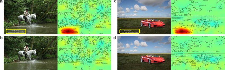
a Linear classification Non-linear classification
b Important features for
individual predictions
Iris setosa (red)
5 5
4 4
sepal width (cm)
sepal width (cm)
sepal
3 3
S2 S2
S 1 S "To detect this boat look
Important features for
1
2 V 2 V
1 1
Iris virginica (green) at the wheelhouse!"
whole ensemble of data
1 1
4 5 6 7 8 4 5 6 7 8
sepal length (cm) sepal length (cm)
Explaining individual classification decisions
Linear classification sepal
Non-linear classification
S1: sepal width S1: sepal width & length Iris versicolor (blue)
S2: sepal width "To detect this boat look "To detect a boat look
S2: sepal width
sepal at the sails!" in the middle of the picture!"
V1: sepal width V1: sepal length
...
"To detect this boat look
at the bow!"
Figure 1: Explanation of a linear and non-linear classifier. (a) In linear models the importance of each feature is the
same for every data point. It can be expressed in the weight vector perpendicular to the decision surface where more
important features have larger weights. In nonlinear models the important features can be different for every data
point. In this example the classifiers are trained to separate “Iris setosa” (red dots) from “Iris virginica” (green dots)
and “Iris versicolor” (blue dots). The linear model for all examples uses the sepal width as discriminative feature,
whereas the non-linear classifier uses different combinations of sepal width and sepal length for every data point. (b)
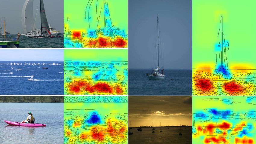
Different features can be important (here for a deep neural network) to detect a ship in an image. For some ships,
the wheelhouse is a good indicator for class “ship”, for others the sails or the bow is more important. Therefore
individual predictions exhibit very different heatmaps (showing the most relevant locations for the predictor). In
feature selection, one identifies salient features for the whole ensemble of training data. For ships (in contrast to e.g.
airplanes) the most salient region (average of individual heatmaps) is the center of the image.
While it is broadly accepted that the nonlinear machine learning (ML) methods being used as predictors
to maximize some prediction accuracy, are effectively (with few exceptions such as shallow decision trees)
black boxes; this intransparency regarding explanation and reasoning is preventing a wider usage of nonlinear
prediction methods in the sciences (see Figure 1a why understanding nonlinear learning machines is difficult).
Due to this black-box character, a scientist may not be able to extract deep insights about what the nonlinear
system has learned, despite the urge to unveil the underlying natural structures. In particular, the conclusion
in many scientific fields has so far been to prefer linear models [1–4] in order to rather gain insight (e.g.
regression coefficients and correlations) even if this comes at the expense of predictivity.
Recently, impressive applications of machine learning in the context of complex games (Atari games [5,6],
Go [7–9], Texas hold’em poker [10]) have led to speculations about the advent of machine learning systems
embodying true “intelligence”. In this note we would like to argue that for validating and assessing machine
behavior, independent of the application domain (sciences, games etc.), we need to go beyond predictive
performance measures such as the test set error towards understanding the AI system.
When assessing machine behavior, the general task solving ability must be evaluated (e.g. by measuring
the classification accuracy, or the total reward of a reinforcement learning system). At the same time it is
important to comprehend the decision making process itself. In other words, transparency of the what and
why in a decision of a nonlinear machine becomes very effective for the essential task of judging whether
the learned strategy is valid and generalizable or whether the model has based its decision on a spurious
correlation in the training data (see Figure 2a). In psychology the reliance on such spurious correlations
is typically referred to as the Clever Hans phenomenon [11]. A model implementing a ‘Clever Hans’ type
2
decision strategy will likely fail to provide correct classification and thereby usefulness once it is deployed in
the real world, where spurious or artifactual correlations may not be present.
     While feature selection has traditionally explained the model by identifying features relevant for the whole
ensemble of training data [12] or some class prototype [13–16], it is often necessary, especially for nonlinear
models, to focus the explanation on the predictions of individual examples (see Figure 1b). A recent series of
work [13, 17–22] has now begun to explain the predictions of nonlinear machine learning methods in a wide
set of complex real-world problems (e.g. [23–26]). Individual explanations can take a variety of forms: An
ideal (and so far not available) comprehensive explanation would extract the whole causal chain from input to
output. In most works, reduced forms of explanation are considered, typically, collection of scores indicating
the importance of each input pixel/feature for the prediction (note that computing an explanation does not
require to understand neurons individually). These scores can be rendered as visual heatmaps (relevance
maps) that can be interpreted by the user.
     In the following we make use of this recent body of work, in particular, the layer-wise relevance propaga-
tion (LRP) method [18] (cf. Section 4.1), and discuss qualitatively and quantitatively, for showcase scenarios,
the effectiveness of explaining decisions for judging whether learning machines exhibit valid and useful prob-
lem solving abilities. Explaining decisions provides an easily interpretable and computationally efficient way
of assessing the classification behavior from few examples (cf. Figure 2a). It can be used as a complement or
practical alternative to a more comprehensive Turing test [27] or other theoretical measures of machine intel-
ligence [28–30]. In addition, the present work contributes by further embedding these explanation methods
into our framework SpRAy (spectral relevance analysis) that we present in Section 4. SpRAy, on the basis
of heatmaps, identifies in a semi-automated manner a wide spectrum of learned decision behaviors and thus
helps to detect the unexpected or undesirable ones. This allows one to systematically investigate the clas-
sifier behavior on whole large-scale datasets — an analysis which would otherwise be practically unfeasible
with the human tightly in the loop. Our semi-automated decision anomaly detector thus addresses the last
mile of explanation by providing an end-to-end method to evaluate ML models beyond test set accuracy or
reward metrics.

2     Results
2.1    Identifying valid and invalid problem-solving behaviors
In this section we will investigate several showcases that demonstrate the effectiveness of explanation methods
like LRP and SpRAy for understanding and validating the behavior of a learned model.
    First, we provide an example where the learning machine exploits an unexpected spurious correlation in
the data to exhibit what humans would refer to as “cheating”. The first learning machine is a model based
on Fisher vectors (FV) [31, 32] trained on the PASCAL VOC 2007 image dataset [33] (see Section E). The
model and also its competitor, a pretrained Deep Neural Network (DNN) that we fine-tune on PASCAL
VOC, show both excellent state-of-the-art test set accuracy on categories such as ‘person’, ‘train’, ‘car’, or
‘horse’ of this benchmark (see Table 3). Inspecting the basis of the decisions with LRP, however, reveals for
certain images substantial divergence, as the heatmaps exhibiting the reasons for the respective classification
could not be more different. Clearly, the DNN’s heatmap points at the horse and rider as the most relevant
features (see Figure 14). In contrast, FV’s heatmap is most focused onto the lower left corner of the image,
which contains a source tag. A closer inspection of the data set (of 9963 samples [33]) that typically humans
never look through exhaustively, shows that such source tags appear distinctively on horse images; a striking
artifact of the dataset that so far had gone unnoticed [34]. Therefore, the FV model has ‘overfitted’ the
PASCAL VOC dataset by relying mainly on the easily identifiable source tag, which incidentally correlates
with the true features, a clear case of ‘Clever Hans’ behavior. This is confirmed by observing that artificially
cutting the source tag from horse images significantly weakens the FV model’s decision while the decision
of the DNN stays virtually unchanged (see Figure 14). If we take instead a correctly classified image of a
Ferrari and then add to it a source tag, we observe that the FV’s prediction swiftly changes from ‘car’ to
‘horse’ (cf. Figure 2a) a clearly invalid decision (see Section E and Figures 15-20 for further examples and

                                                        3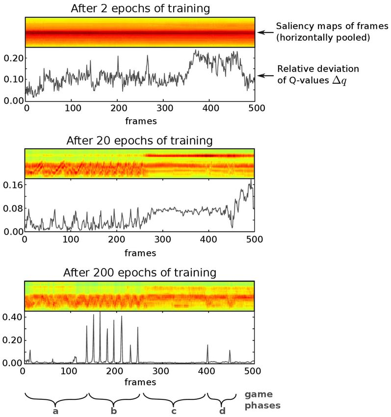
a          Horse-picture from Pascal VOC data set                                                 Artificial picture of a car

                                                             Source tag
                                                              present

                                                             Classified
                                                             as horse

                                                             No source
                                                            tag present

                                                            Not classified
                                                              as horse

     b               Pinball - Relevance during game play                   c                        Breakout - Relevance during training

                                                                                                                                    a Ball
                                                                                                                                    b Paddle

                                                                                Relative relevance
                                                                     x4                                                             c Tunnel

                                                                                                            50        100          150         200
                                                                                                                             Training epoch

Figure 2: Assessing problem-solving capabilities of learning machines using explanation methods. (a) The Fisher
vector classifier trained on the PASCAL VOC 2007 data set focuses on a source tag present in about one fifth of the
horse figures. Removing the tag also removes the ability to classify the picture as a horse. Furthermore, inserting
the tag on a car image changes the classification from car to horse. (b) A neural network learned to play the Atari
Pinball game. The model moves the pinball into a scoring switch four times to activate a multiplier (indicated as
symbols marked in yellow box) and then maneuvers the ball to score infinitely. This is done purely by “nudging the
table” and not by using the flippers. In fact, heatmaps show that the flippers are completely ignored by the model
throughout the entire game, as they are not needed to control the movement of the ball. (c) Development of the
relative relevance of different game objects in Atari Breakout over the training time. Relative relevance is the mean
relevance of pixels belonging to the object (ball, paddle, tunnel) divided by the mean relevance of all pixels in the
frame. Thin lines: 6 training runs. Thick line: average over the 6 runs.

analyses).
    The second showcase example studies neural network models (see Figure 5 for the network architecture)
trained to play Atari games, here Pinball. As shown in [5], the DNN achieves excellent results beyond
human performance. Like for the previous example, we construct LRP heatmaps to visualize the DNN’s
decision behavior in terms of pixels of the pinball game. Interestingly, after extensive training, the heatmaps
become focused on few pixels representing high-scoring switches and loose track of the flippers. A subsequent
inspection of the games in which these particular LRP heatmaps occur, reveals that DNN agent firstly moves
the ball into the vicinity of a high-scoring switch without using the flippers at all, then, secondly, “nudges”
the virtual pinball table such that the ball infinitely triggers the switch by passing over it back and forth,
without causing a tilt of the pinball table (see Figure 2b and Figure 6 for the heatmaps showing this point,
and also Supplementary Video 1). Here, the model has learned to abuse the “nudging” threshold implemented

                                                             4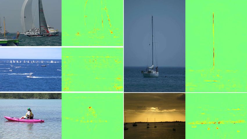
a
             Input Data for "Horse"                     Classifier                       Class Predictions
                                                                                                 "cat"
                                                                                                         "bird" "sheep"
                                                                                          "cow"
                                                                                                    "dog" "aeroplane"
                                                                                       "bicycle"

                                                                                    "sofa" "boat"
                                                                                                    "horse"       "bus"
                                                                                                    "car"     "motorbike"
                                                                                      "bottle"
                                                                                                 "person""pottedplant"
                                                                                       "tvmonitor"        "chair"
                                                                                                                    "train"
                                                                                             "diningtable"

                 Relevance Heatmaps for
                     "Horse" Decision

                 Eigenvalue-Based
                     Clustering

                     Large Eigengaps
                     Small Eigenvalues

                                                                                   Identified Strategies
                                                                                  For Detecting "Horse"

     b                             c                          d                         e

Figure 3: The workflow of Spectral Relevance Analysis. (a) First, relevance maps are computed for data samples
and object classes of interest, which requires a forward and a LRP backward pass through the model (here a Fisher
vector classifier). Then, an eigenvalue-based spectral cluster analysis is performed to identify different prediction
strategies within the analyzed data. Visualizations of the clustered relevance maps and cluster groupings supported
by t-SNE inform about the valid or anomalous nature of the prediction strategies. This information can be used
to improve the model or the dataset. Four different prediction strategies can be identified for classifying images as
“horse”: (b) detect a horse (and rider), (c) detect a source tag in portrait oriented images, (d) detect wooden hurdles
and other contextual elements of horseback riding, and (e) detect a source tag in landscape oriented images.

through the tilting mechanism in the Atari Pinball software. From a pure game scoring perspective, it is
indeed a rational choice to exploit any game mechanism that is available. In a real pinball game, however, the
player would go likely bust since the pinball machinery is programmed to tilt after a few strong movements
of the whole physical machine.
    The above cases exemplify our point, that even though test set error may be very low (or game scores very

                                                          5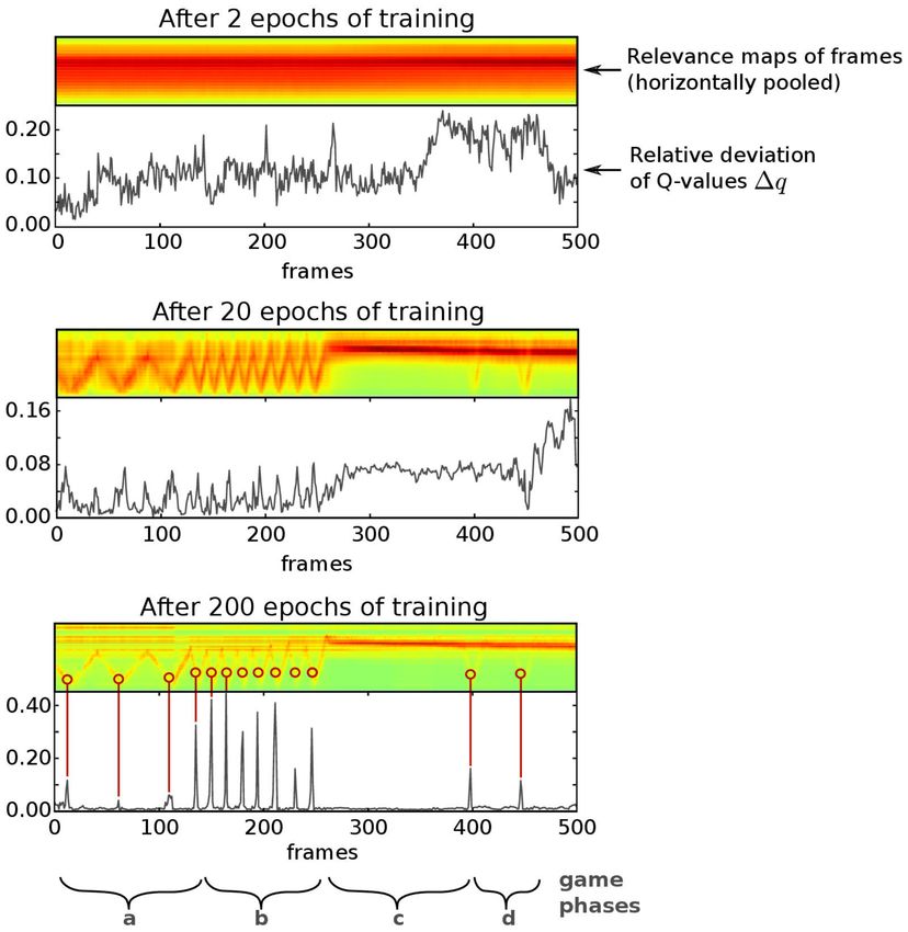
high), the reason for it may be due to what humans would consider as cheating rather than valid problem-
solving behavior. It may not correspond to true performance when the latter is measured in a real-world
environment, or when other criteria (e.g. social norms which penalize such behavior [35]) are incorporated
into the evaluation metric. Therefore, explanations computed by LRP have been instrumental in identifying
this fine difference.
    Let us consider a third example where we can beautifully observe learning of strategic behavior: A
Deep Neural Network playing the Atari game of Breakout [5] (see Table 2 for the investigated network
architectures). We analyze the learning progress and inspect the heatmaps of a sequence of DNN models
in Figure 2c. The heatmaps reveal conspicuous structural changes during the learning process. In the first
learning phase the DNN focuses on ball control, the handle becomes salient as it learns to target the ball and
in the final learning phase the DNN focuses on the corners of the playing field (see Figure 2c). At this stage,
the machine has learned to dig tunnels at the corners (also observed in [5]) – a very efficient strategy also
used by human players. Detailed analyses using the heatmap as a function of a single game and comparison
of LRP to sensitivity analysis explanations, can be found in the Figures 7-13 and in the Supplementary Video
2. Here, this objectively measurable advancement clearly indicates the unfolding of strategic behavior.
    Overall, while in each scenario, reward maximization as well as incorporating a certain degree of prior
knowledge has done the essential part of inducing complex behavior, our analysis has made explicit that
(1) some of these behaviors incorporate strategy, (2) some of these behaviors may be human-like or not
human-like, and (3) in some case, the behaviors could even be considered as deficient and not acceptable,
when considering how they will perform once deployed. Specifically, the FV-based image classifier is likely
to not detect horses on the real-world data; and the Atari Pinball AI might perform well for some time, until
the game is updated to prevent excessive nudging.
    All insights about the classifier behavior obtained up to this point of this study require the analysis of
individual heatmaps by human experts, a laborious and costly process which does not scale well.

2.2    Whole-dataset analysis of classification behavior
Our next experiment uses SpRAy to comprehend the predicting behavior of the classifier on large datasets in
a semi-automated manner. Figure 3a displays the results of the SpRAy analysis when applied to the horse
images of the PASCAL VOC dataset (see also Figures 22 and 23). Four different strategies can be identified
for classifying images as “horse”: 1) detect a horse and rider (Figure 3b), 2) detect a source tag in portrait
oriented images (Figure 3c), 3) detect wooden hurdles and other contextual elements of horseback riding
(Figure 3d), and 4) detect a source tag in landscape oriented images (Figure 3e). Thus, without any human
interaction, SpRAy provides a summary of what strategies the classifier is actually implementing to classify
horse images. An overview of the FV and DNN strategies for the other classes and for the Atari Pinball and
Breakout game can be found in Figures 26-28 and 33-35, respectively.
    The SpRAy analysis could furthermore reveal another ‘Clever Hans’ type behavior in our fine-tuned
DNN model, which had gone unnoticed in previous manual analysis of the relevance maps. The large
eigengaps in the eigenvalue spectrum of the DNN heatmaps for class “aeroplane” indicate that the model
uses very distinct strategies for classifying aeroplane images (see Figure 26). A t-SNE visualization (Figure
28) further highlights this cluster structure. One unexpected strategy we could discover with the help of
SpRAy is to identify aeroplane images by looking at the artificial padding pattern at the image borders,
which for aeroplane images predominantly consists of uniform and structureless blue background. Note that
padding is typically introduced for technical reasons (the DNN model only accepts square shaped inputs),
but unexpectedly (and unwantedly) the padding pattern became part of the model’s strategy to classify
aeroplane images. Subsequently we observe that changing the manner in which padding is performed has a
strong effect on the output of the DNN classifier (see Figures 29-32).
    We note that while recent methods (e.g. [36]) have characterized whole-dataset classification behavior
based on decision similarity (e.g. cross-validation based AP scores or recall), the SpRAy method can pinpoint
divergent classifier behavior even when the predictions look the same. The specificity of SpRAy over previous
approaches is thus its ability to ground predictions to input features, where classification behavior can be

                                                      6
more finely characterized. A comparison of both approaches is given in Section E and Supplementary Figures
24 and 25.

3     Discussion
Although learning machines have become increasingly successful, they often behave very differently from
humans [37, 38]. Commonly discussed ingredients to make learning machines act more human-like are
e.g. compositionality, causality, learning to learn [39–41], and also an efficient usage of prior knowledge or
invariance structure (see e.g. [42–44]). Our work adds a dimension that has so far not been a major focus of
the machine intelligence discourse, but that is instrumental in verifying the correct behavior of these models,
namely explaining the decision making. We showcase the behavior of learning machines for two application
fields: computer vision and arcade gaming (Atari), where we explain the strategies embodied by the respective
learning machines. We find a surprisingly rich spectrum of behaviors ranging from strategic decision making
(Atari Breakout) to ‘Clever Hans’ strategies or undesired behaviors, here, exploiting a dataset artifact (tags
in horse images), a game loophole (nudging in Atari Pinball), and a training artifact (image padding). These
different behaviors go unnoticed by common evaluation metrics, which puts a question mark to the current
broad and sometimes rather unreflected usage of machine learning in all application domains in industry
and in the sciences.
    With the SpRAy method we have proposed a tool to systematize the investigation of classifier behavior
and identify the broad spectrum of prediction strategies. The SpRAy analysis is scalable and can be applied to
large datasets in a semi-automated manner. We have demonstrated that SpRAy easily finds the misuse of the
source tag in horse images, moreover and unexpectedly, it has also pointed us at a padding artifact appearing
in the final fine-tuning phase of the DNN training. This artifact resisted a manual inspection of heatmaps
of all 20 PASCAL VOC classes, and was only later revealed by our SpRAy analysis. This demonstrates
the power of an automated, large-scale model analysis. We believe that such analysis is a first step towards
confirming important desiderata of AI systems such as trustworthiness, fairness and accountability in the
future, e.g. in context of regulations concerning models and methods of artificial intelligence, as via the
General Data Protection Regulation (GDPR) [45, 46]. Our contribution may also add a further perspective
that could in the future enrich the ongoing discussion, whether machines are truly “intelligent”.
    Finally, in this paper we posit that the ability to explain decisions made by learning machines allows us
to judge and gain a deeper understanding of whether or not the machine is embodying a particular strategic
decision making. Without this understanding we can merely monitor behavior and apply performance
measures without possibility to reason deeper about the underlying learned representation. The insights
obtained in this pursuit may be highly useful when striving for better learning machines and insights (e.g. [47])
when applying machine learning in the sciences.

4     Methods
4.1    Layer-wise relevance propagation
Layer-wise relevance propagation (LRP) [18] is a method for explaining the predictions of a broad class of
ML models, including state-of-the-art neural networks and kernel machines. It has been extensively applied
and validated on numerous applications [23, 26, 34, 48–50]. The LRP method decomposes the output of the
nonlinear decision function in terms of the input variables, forming a vector of input features scores that
constitutes our ‘explanation’. Denoting x = (x1 , . . . , xd ) an input vector and f (x) the prediction at the
output of the network, LRP produces a decomposition R = (R1 , . . . , Rd ) of that prediction on the input
variables satisfying
                                             Pd
                                               p=1 Rp = f (x).                                             (1)

                                                       7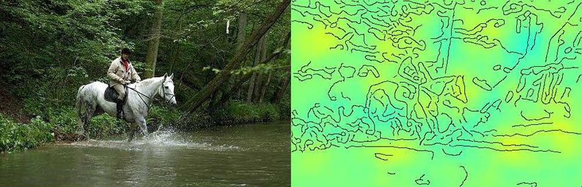
Unlike sensitivity analysis methods [51], LRP explains the output of the function rather than its local
variation [52] (see Section C for more information on explanation methods).
   The LRP method is based  P on a backward propagation mechanism applying uniformly to all neurons in
the network: Let aj =P    ρ( Pi ai wij + bj ) be one such neuron. Let i and j denote the neuron indices at
consecutive layers, and i , j the summation over all neurons in these respective layers. The propagation
mechanism of LRP is defined as
                                                    X zij
                                               Ri =     P       Rj .                                   (2)
                                                      j   i zij

where zij is the contribution of neuron i to the activation aj , and typically depends on the activation ai and
the weight wij . The propagation rule is applied in a backward pass starting from the neural network output
f (x) until the input variables (e.g. pixels) are reached. Resulting scores can be visualized as a heatmap of
same dimensions as the input (see Figure 4).
    LRP can be embedded in the theoretical framework of deep Taylor decomposition [22], where some of
the propagation rules can be seen as particular instances. Note that LRP rules have also been designed for
models other than neural networks, in particular, Bag of Words classifiers, Fisher vector models, and LSTMs
(more information can be found in the Section C and Table 1).

4.2    Spectral relevance analysis
Explanation techniques enable inspection of the decision process on a single instance basis. However, screen-
ing through a large number of individual explanations can be time consuming. To efficiently investigate
classifier behavior on large datasets, we propose a technique: Spectral Relevance Analysis (SpRAy). SpRAy
applies spectral clustering [53] on a dataset of LRP explanations in order to identify typical as well as
atypical decision behaviors of the machine learning model, and presents them to the user in a concise and
interpretable manner.
     Technically, SpRAy allows one to detect prediction strategies as identifiable on frequently reoccurring
patterns in the heatmaps, e.g., specific image features. The identified features may be truly meaningful
representatives of the object class of interest, or they may be co-occurring features learned by the model but
not intended to be part of the class, and ultimately of the model’s decision process. Since SpRAy can be
efficiently applied to a whole large-scale dataset, it helps to obtain a more complete picture of the classifier
behavior and reveal unexpected or ‘Clever Hans’ type decision making.
     The SpRAy analysis is depicted in Figure 3 (see also Section F) and consists of four steps: Step 1:
Computation of the relevance maps for the samples of interest. The relevance maps are computed with
LRP and contain information about where the classifier is focusing on when classifying the images. Step 2:
Downsizing of the relevance maps and make them uniform in shape and size. This reduction of dimensionality
accelerates the subsequent analysis, and also makes it statistically more tractable. Step 3: Spectral cluster
analysis (SC) on the relevance maps. This step finds structure in the distribution of relevance maps, more
specifically it groups classifier behaviors into finitely many clusters (see Figure 21 for an example). Step 4:
Identification of interesting clusters by eigengap analysis. The eigenvalue spectrum of SC encodes information
about the cluster structure of the relevance maps. A strong increase in the difference between two successive
eigenvalues (eigengap) indicates well-separated clusters, including atypical classification strategies. The few
detected clusters are then presented to the user for inspection. Step 5 (Optional): Visualization by t-
Stochastic Neighborhood Embedding (t-SNE). This last step is not part of the analysis strictly speaking,
but we use it in the paper in order to visualize how SpRAy works.
     Since SpRAy aims to investigate classifier behavior, it is applied to the heatmaps and not to the raw
images (see Figures 23, 27 and 28 for comparison).

                                                       8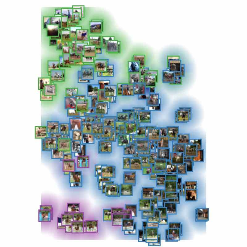
Code availability
Source code for LRP and sensitivity analysis is available at https://github.com/sebastian-lapuschkin/
lrp_toolbox. Source code for Spectral Clustering and t-SNE as used in the SpRAy method is available from
the scikit-learn at https://github.com/scikit-learn/scikit-learn. Source code for the Reinforcement-
Learning-based Atari Agent is available at https://github.com/spragunr/deep_q_rl. Source code for the
Fisher Vector classifier is available at http://www.robots.ox.ac.uk/~vgg/software/enceval_toolkit.
Our fine-tuned DNN model can be found at
https://github.com/BVLC/caffe/wiki/Model-Zoo#pascal-voc-2012-multilabel-classification-model.

Data availability
The datasets used and analyzed during the current study are available from the following sources.
PASCAL VOC 2007: http://host.robots.ox.ac.uk/pascal/VOC/voc2007/#devkit.
PASCAL VOC 2012: http://host.robots.ox.ac.uk/pascal/VOC/voc2012/#devkit.
Atari emulator: https://github.com/mgbellemare/Arcade-Learning-Environment.

Appendix
A     Introduction
AI systems are able to solve an increasing number of complex tasks. They occasionally exceed human
performance spectacularly in tasks as diverse as face recognition [54], traffic sign classification [55], reading
subway plans [56], understanding quantum many-body systems [43,44,47,57] or playing games such as Atari
2600 games [5, 6], Go [7, 8], Texas hold’em poker [10] or Super Smash Bros. [58]. This impressive progress is
largely owed to recent advances in deep learning, i.e., a class of end-to-end trainable, brain-inspired models
with multiple (deep) layers of unfolding representations. Not surprisingly, these high-performance methods
have quickly found their way out of research labs and are attracting much attention in the industry and the
media. While these algorithms seem to clearly exhibit outstanding performance in the respective tasks, there
is an ongoing debate on “intelligence” in AI systems in general [28, 37, 59–61], how to measure it and what
could be the limits thereof. Amongst others this discussion aims to elucidate the defining ingredients for
truly human-like learning such as compositionality, representation and how to include prior knowledge about
the world [37]. With this work we would like to add interpretability to this discussion as it is instrumental
in judging and validating the behavior of these systems.
    Let us first briefly roll out aspects of the current discussion. The authors of [37, 38] analyze key aspects
of human-like learning. A major difference between machine and human learning is that humans (even
infants) are equipped with a “start-up” software [62, 63] consisting of a priori representation about objects
and physics [64, 65] and about other agents [66, 67]. This enables them to quickly learn to interact with the
environment, to reason about future world states (e.g, position of objects in space) and to understand other
people’s goals, beliefs and strategies. Since such priors or also the knowledge about invariances [68] are usually
not available to a machine unless coded (see e.g. [43, 68]), learning them takes significantly longer, requires
orders of magnitude more examples and the learned concepts are less transferable to other tasks. Recently,
Lake et al. [41] proposed a learning machine that implements some of the human learning abilities and is
able to learn new concepts from just a single example. The model brings together three important learning
principles which have been intensively studied in cognitive science [39, 40] and are regarded as indispensable
ingredients of human learning. These principles are (1) compositionality, i.e., the ability to build rich concepts
from simpler primitives, (2) causality, i.e., the ability to model and infer the causal structure of the world,
and (3) learning to learn, i.e., the ability to develop hierarchical priors which simplify learning new concepts
from previous experience. Lake et al. [41] incorporated these principles into a Bayesian program learning
framework and showed on a restricted problem set, e.g., one-shot classification of handwritten characters,
that their model achieves human-level performance and outperforms recent deep learning algorithms. Future

                                                        9
generations of neural networks incorporating above principles may be able to approach human learning even
in more realistic scenarios.
     A further important aspect of human intelligence termed computational rationality was discussed in [69].
Humans are adapted to interact with a dynamically changing, partially unknown and uncertain environment
and thus are able to identify decisions with high expected utility while taking trade-offs in effort, precision,
and timeliness of computations. Finding appropriate trade-offs and optimally allocating scarce resources is
a difficult task which requires intelligence on a “meta-level”. Recently, researchers started to bring these
aspects to deep learning by incorporating mechanism such as attention [70] or memory [56] into neural
network models. Future AI systems that aim to interact with the real-world to a greater extent, may
possibly have to fully implement computational rationality in order to be able to make meta-level decisions
to better and more efficiently regulate base-level inferences.
     A crucial aspect of human behavior, and the main focus of this paper, is the ability to explain [71, 72].
It facilitates practical learning, e.g., in a student-teacher context, by not only providing the solution to a
problem but also the description of how to solve the problem, what features to rely on etc. Furthermore,
explanations have an important social role, because they enable to comprehend and rationalize other indi-
viduals’ decisions, they also help establishing trust (e.g., doctor explains therapy to patient) and they are
indispensable when the correctness of a decision needs to be verified. Until recently, deep neural networks
and other complex, non-linear learning machines have been mainly used in a black-box manner, providing
little information on what aspect of the input data supports the actual prediction for a single sample. This
black-box behavior can amount to a major disadvantage and prevent the application of state-of-the-art AI
technology in critical application domains. For instance, in medical diagnosis the ability to verify a deci-
sion made by an AI system is crucial for a medical professional as a wrong decision can cause threats to
human life [73]. Additionally, black-box systems are of limited value in the sciences, where it is crucial to
ensure that the learned model is biologically, chemically or physically plausible or ideally contributes to a
better understanding of the scientific problem [47]. In practice, if the learning machine is interpretable, we
can visualize what it has learned, how it arrives at its conclusions and whether its task-solving strategy is
meaningful, sensible and comprehensible from a human point of view. Also it can help confirming other
important desiderata of AI systems such as fairness or accountability [74–76].
     We will demonstrate in this work that state-of-the-art AI systems exhibit unexpected and to human
standards not necessarily meaningful problem solution strategies. In particular, we would like to argue that
this undesired behavior often goes unnoticed if AI models are not interpreted. Therefore, we will introduce
in Section C recent techniques which allow to explain individual predictions of black-box AI models. Then,
these techniques will be showcased in Section D and E, by performing a detailed analysis of the behavior of
Atari agents and image classifiers. Finally, we contribute in Section F a novel procedure for identifying erratic
behavior of these systems in a semi-automated manner. Overall, our results demonstrate that interpretability
provides a very effective way of assessing the validity and dependability of AI systems and we are convinced
that it will also help us design more human-like AI systems in the future.

B     Background
We will now specifically focus on deep convolutional networks [77, 78], which incorporate the principles of
hierarchy and shift-invariance. They have scored commanding successes in the venues of strategic games [5,7,
58,79], image classification [78], face [80,81] recognition, speech recognition [82] and e.g. physics [47,83]. In the
following we briefly introduce how neural networks work and how they can be combined with reinforcement
learning to play arcade games.

Neural Networks Neural networks are a highly nonlinear, modular and hierarchical approach to learning
[84–86]. The advent of GPU accelerated training [87] and the availability of performant deep learning
frameworks [88–92], as well as large datasets [33, 93–97] lead to unprecedented accuracy in a variety of
tasks [5, 7, 78, 80, 98, 99]. Neural networks are composed of multiple layers, each consisting of a linear and a

                                                         10
non-linear transformation,
(l+1)
X (l) (l) (l)
xj = g w x + bj ,
j,k k (3)
j
where g is a non-linear function, e.g. sigmoid function, hyperbolic tangent or a rectifier function [100]. The
universal approximation theorem ensures that any continuous function on a compact interval of Rn can be
approximated by a neural network to an arbitrary precision [101–103].
Although only one hidden layer is strictly necessary, having a deeper structure allows this approximation
to be more efficient in the number of neurons required [104]. State-of-the-art deep neural networks achieve
astounding results with many hidden layers, some numbering eight [78], twenty-two [105] or even more than
one hundred [106] layers. The deep structure allows the networks to operate on conceptual levels with each
layer processing more complex features (e.g. edges → corners → rectangles → boxes → cars) mirroring
abstraction levels similar to the human brain [107, 108]. It can be shown that from layer to layer, networks
compress information and enhance the signal-to-noise ratio (see [109, 110]).
There are three major learning paradigms for DNN’s, each corresponding to a particular abstract learning
task, i.e. supervised learning, unsupervised learning and reinforcement learning. In this work we focus on
supervised and reinforcement learning to train the agents and evaluate their decisions for a better under-
standing.
Supervised Learning In supervised learning the goal is to infer a function f from a labeled training
dataset consisting of the samples xi and their label yi . If the labels only take discrete values, then we refer to
the learning problem as classification problem, otherwise it is called a regression problem. Often f belongs to
a parameterized class of functions, e.g., neural networks with a particular architecture, then the learning task
reduces to finding the “optimal” parameters (w.r.t. a specific loss). In practice, algorithms such as stochastic
gradient descent [111] and variants of it such as Adam [112] are used for this optimization. After training we
can use function f to estimate the predictions for unseen samples (i.e., testing phase) in order to approximate
its generalization ability. In Section E we will analyze and compare the generalization performance and task-
solving strategy of two powerful systems for image categorization — a typical supervised learning task.
Reinforcement Learning In a typical reinforcement learning setting, an agent is trained without explic-
itly labelled data, via interaction with the environment only. At each time step t of the training process, the
agent to be trained performs a preferred
P action at based on a state st and receives a reward rt with the goal
to maximize the long term reward t rt by adapting the model parameters determining which action is to
be chosen given an input.
Recently, a convolutional neural network was trained to play simple Atari video games with visual input
on a human-like level [5]. Using Q-learning [113], a model-free reinforcement learning technique, a network
has been trained to fit an action-value function. The Q-learning setup consists of three elements:
1. the Arcade Learning Environment [114] that takes an action as input, advances the game and
returns a visual representation of the game and a game score,
2. the Neural Network that predicts a long-term reward, the so-called Q-function Q(s, a; θ), for a game
visual for every possible action a, and, lastly,
3. the Replay Memory that saves observed game transitions during the training as tuples (state,
action, reward, next state), from now on (st , at , rt , st+1 ).
To update the network, Mnih et al. [5] make use of the fact that the optimal Q-function, Q∗ must obey
the Bellman equation [115]
∗ ∗
Q (st , at ) = Est+1 rt + γ max Q (st+1 , at+1 ) st , at , (4)
at+1
11which can be used to train the network by choosing the cost function as the squared violation of the Bellman
equation. The expectation value is approximated by the sum over a batch of game transitions B drawn
uniformly at random from the replay memory.
X h i2
0 0
C(θ) = Q(s, a; θ) − r + γ max
0
Q(s , a ; θ) .
a
(s,a,r,s0 )∈B
The agent is trained by alternating three steps. First, it explores its environment using the actions that
promise the highest long-term reward according to its own estimations. Second, it records the observations
it encounters and saves the game transitions in the replay memory, potentially replacing older transitions.
Third, one trains the network to predict the long-term reward by drawing batches from the replay memory
and updating the cost functional.
The interplay of environment, network and memory is a convoluted process where convergence is not
guaranteed [116]. Methods to explain the network decisions can be used to chart the development of the
neural agent even at stages where it is not yet able to successfully interact with the environment. As we will
see later, this will be useful to correct the network architecture early on.
C Understanding AI Systems
Nonlinear learning methods such as neural networks are often (but falsely) considered as black boxes. One
approach to assess the quality of these learning machines is to observe the model’s behavior on an independent
test dataset and from that draw conclusions about it’s problem solving strategies. Although theoretically
valid, this approach may be very cumbersome or even practically impossible for AI systems, because eval-
uating the responses of the system to all possible variations of the input requires huge amount of testing
(curse of dimensionality). In practice test datasets are often small and not representative. More advanced
approaches exist for measuring or defining the capabilities of AI systems (e.g., [28–30, 117]), however, these
tests rather focus on assessing the system’s performance in solving various tasks than on understanding the
decision process (in particular the single decision) itself.
In this work we argue that to fully understand the quality of a learning machine, its intrinsic nonlinear
decision making process needs to be made accessible to human judgment. Understanding the basis of
decisions is desirable for many reasons:
(1) In cases where we know what the decision should be based on, we can judge the soundness (according
to human standards) of the decision process.
(2) If we do not know what the decision should be based on but we can trust the system, we may infer
new domain knowledge. For example, Vidovic et al. [118] use an accomplished SVM classifier that
predicts protein splice sites from large gene sequences to also explain which base pair motifs in genes
were decisive for the classification. This can potentially increase our understanding or at least narrow
down interesting domains for further, more informed, research.
(3) Even if we can not make sense of the explanations, e.g., because we are not domain experts, it is still
possible to use this extra information for detection of erratic behavior of the AI system (see Section F).
We provide an example of such erratic behavior in Section E, where we train a Fisher vector classifier
which unintentionally bases its decision on a spurious correlation. For images showing horses, the
model has learned to dominantly decide based on the presence of a copyright watermark on one of the
corners of the images. Of course, in the world portrayed by an artifactual dataset it is completely valid
to assume that horses are connected to the existence of a source tag. But from human perspective
this is the Clever Hans phenomenon [11] well known in comparative psychology, i.e., the system uses a
spurious correlation1 to solve the problem without understanding the problem. It is obvious that the
1 The Orlov Trotter horse claimed to perform arithmetic and other intellectual tasks, but actually was watching the reactions
of his trainer.
12learning system in our case does not truly understand the concept of a horse.
There is also an interesting phenomenon described in the literature, the AI effect [60], saying that
everytime an AI system solves a problem which has been regarded as an intelligence task, e.g., playing
checkers or chess, it is is not regarded as being “intelligent” after some time, but solving the problem is
regarded as rather computation. Thus AI systems (e.g., alphaGo [7], DeepStack [10] or subway plan reading
system [56]) which are regarded intelligent today, may be not regarded as intelligent anymore in the near
future.
C.1 Explaining Classification Decisions
In the context of image recognition, classification decisions can be explained by tracing the model decision
down to the input pixels. The resulting explanation takes the form of an image of the same format as the
input image, for which the content provides visualizable feedback on the classification decision of the learned
model (see e.g. [52]). In particular, it will reveal which part of the image is important for classification, and
more precisely, which pattern in the image causes the neural network to decide.
The first approaches to extract interpretable visual patterns from a classifier’s decision were based on
Sensitivity Analysis [13,19,51]. These methods rely on the gradient of the decision function and identify input
variables (e.g., pixels) which maximally strengthen or weaken the classifier decision signal when changed.
Strictly speaking these methods do not explain the prediction (“what made the classifier arrive at it’s
decision”), but analyze the local variation of the classification function (see [52] for more discussion). Other
more recent techniques [17,20,119–122] extract visual patterns associated to the decision of deep convolutional
neural networks by using different heuristic criteria (e.g., occlusion, perturbation, sampling or deconvolution).
A principled analysis technique for explaining decisions of complex models such as deep neural networks or
bag-of-words-type classifiers has emerged with Layer-wise Relevance Propagation (LRP) [18, 22]. We will
describe this technique below and use it throughout the experiments of this paper. A theoretical foundation
of LRP, called deep Taylor decomposition, can be found in [22]. Explanation methods were successfully
applied to a wide set of complex real-world problems such as the analysis of faces [81, 123, 124], EEG
and fMRI data [23, 50], human gait [48], videos [125], speech [126], reinforcement learning [25], biological
data [127], text [26, 128, 129], or comparing human and algorithm behavior in the context of visual question
answering [130].
C.2 Pixel-Wise Decompositions
A natural way of explaining a classifier’s decision is to decompose its output as a sum of pixel-wise scores
representing the relevance of each pixel for the decision. More precisely, denoting by Rf the output of the
neural network, and Rp the relevance of pixel p, one requires that the following conservation property holds
P
p Rp = Rf ,
where the sum runs over all pixels in the image. Several methods, including LRP, perform such decomposition
[18, 22, 131, 132]. An advantage of the decomposition framework is versatility: If needed, one can directly
recompute the analysis at a coarser level by aggregating relevance scores according to a partition of the pixel
space [133]. For example, denoting by P a particular region of the image (e.g. its center), we can compute
the total relevance for that region as P
RP = p∈P Rp .
while
P still satisfying the coarser conservation property when summing over all regions of the partition:
P P = Rf . This aggregation property is useful in our study to be able to produce height-aggregated
R
heatmaps, that we can plot as a function of time, thus, allowing to monitor the evolution of the agent
attention for the considered Atari games. The aggregation property is also used implicitly to sum relevance
over the RGB channels of the pixels, and thus produce a single score per pixel.
13Layer-wise Relevance Propagation (LRP) forward pass backward pass
input
DNN
heatmap
layer l layer l+1 layer l layer l+1
Figure 4: Left: Overview of the LRP method. The input image is propagated in a neural network, which classifies
it as “boat”. The classification score is backpropagated in the network, leading to individual pixel-wise relevance
scores that can be visualized as a heatmap. Right: Details of the forward and backward passes for a small portion of
the neural network.
Decomposition methods can be subdivided in three categories: (1) structure approaches, where the
function itself has the particular summation structure, and where individual pixel-wise contributions can
be identified as the summands of the function [131], (2) analytic approaches, where a local analysis of the
function is performed, and where pixel-wise contributions can be identified as linear terms of some local
function expansion [13, 18], (3) propagation approaches [18, 22, 132, 134], where the model is assumed to
describe a directed computational graph, where the output score is propagated through the network under
local conservation constraints until the pixels are reached.
C.3 Layer-Wise Relevance Propagation
We present here the Layer-wise Relevance Propagation (LRP) approach proposed by [18] for obtaining a
pixel-wise decomposition of the model decision and use this technique throughout all experiments of the
paper. LRP uses a propagation approach and is general enough to apply to most of the state-of-the-art
architectures for image classification or neural reinforcement learning, including in particular AlexNet [78],
or Atari-based neural networks [5], and can also be applied to other types of models such as Fisher vector
with SVM classifiers or LSTMs [135, 136]. LRP assumes that the decision function can be decomposed as a
feed-forward graph of neuron computations of type
P
xj = g i xi wij + bj ,
where g is some monotonically increasing nonlinear function (e.g. the ReLU nonlinearity), xi are the neuron
inputs, xj is the neuron activation, and where wij and bj are learned weights and bias parameters. The
propagation behavior of LRP can be characterized by looking at a single neuron: The relevance Rj received
by neuron j from the upper layers must be redistributed to its incoming neurons in the lower layer. For this,
we produce messages Ri←j that satisfy a local conservation property:
P
i Ri←j = Rj
The exact definition of LRP rule is dependent on the neuron type, and its position in the architecture,
however, the message can generally be written as
qij
Ri←j = P Rj ,
i qij
14where qij is a measure of contribution of neuron i to activating neuron j. The relevance score assigned to the
neuron i is subsequently obtained by pooling all relevance messages coming from the higher-layer neurons
to which neuron i contributes: P X qij
Ri = j Ri←j = P Rj
j i qij
The intuition behind this propagation method is that a neuron is defined as relevant if it contributes to
neurons that are relevant themselves. The relevance propagation procedure is iteratively applied from the
top layer down to the pixel layer, at which point the procedure stops. The method is illustrated in Figure
4; for theoretical background see [22]. LRP toolboxes are described in [137, 138].
A possible propagation rule results from defining contributions as the positive part of the product between
the neuron input and the weights qij = (xi wij )+ where ()+ indicates the positive part. qij can be interpreted
as the amount by which neuron i excites neuron j. This rule was advocated by [18, 22, 134], is easy to
implement and particularly suitable for neural networks with ReLU nonlinearities. In this context, this rule
is an instance of the more general αβ-rules proposed by [18]. In practice, the rule can be replaced by other
rules (e.g. the αβ-rules, the -rule, the w2 -rule, or the “flat”-rule) all based on the same local relevance
conservation principles, but with different characteristics such as sparsity, amount of negative evidence, or
domain of applicability. An overview of these rules is given in Table 1, where we use the shortcut notation
zij = xi wij and where we define the map σ : t → t + · sign(t). Finally, max-pooling layers are treated in
this paper by redirecting all relevance to the neuron in the pool that has the highest activation. The Caffe
reference model [90], as used for image categorization in Section E, employs local renormalization layers.
These layers are treated with an approach based on Taylor expansion [139]. Pixel-wise relevance is obtained
by pooling relevance over the RGB components of each pixel.
Table 1: Formula and usage of various LRP-rules. The αβ-rule is used together with flat-weight- or w2 -method for
the neural agents. The -rule is used for the Fisher vectors (FV).
LRP rule Formula Used for
z−
z+
- DNN in [18, 34, 140]
αβ-rule Ri←j = α P ij + + β P ij − Rj
i zij i zij - Atari agents.
2 w2
w -rule Ri←j = P ij 2 Rj - Atari agents (bottom layers)
i wij
z
-rule Ri←j = Pij R - FV top layer in [34, 140]
σ( i zij ) j
P1
- FV local descriptors [18, 34]
flat rule Ri←j = 1
Rj
i - Atari agents (bottom layers)
C.4 Experiments
We analyze the decision process of convolutional neural networks in two different machine intelligence tasks,
reinforcement learning for arcade video games and supervised image classification. In the first task a convo-
lutional neural network is trained to play simple computer games. We explain the decisions of the network
using LRP and visualize the relevance for different game objects. We visualize which game objects the
network focuses on and how this corresponds to the current game situation and the learned strategy for
the games of Breakout and Video Pinball for the Atari 2600. Taking this approach further, we monitor the
importance attributed by the learning machine to different game objects as a function of the training time
and quantify changes in the model’s behavior that are not apparent by monitoring the game score.
Second, we analyze machine behavior for a popular computer vision task; here two ML models are trained
to classify images of the Pascal VOC dataset [33]. Interestingly and anecdotally, one of them, a Fisher vector-
based classifier trained to classify images as horses or non-horses, is shown to rely its decisions on a spurious
correlation: a copyright watermark that accidentally and undetected by the computer vision community
persisted in this highly popular benchmark. For the classification of ships the classifier is mostly focused on
15Input Conv1 Conv2 Conv3 FC1 FC2
8 4 3
8 4 3
84
4
512
84
4 32 64 64
Figure 5: The Atari Network architecture. The network consists of three convolutional layers (Conv) and two fully
connected layers (FC). All layers comprise a ReLU-nonlinearity except for the last FC layer. The network output
corresponds to a vector that predicts the Q-function for every possible action, in this example “go left”, “go right”,
“fire” and “do nothing”.
the presence of water in the bottom half of an image. Removing the copyright tag or the background results
in a drop of predictive capabilities. A deep neural network, pre-trained in the ImageNet dataset [93], instead
shows none of these shortcomings.
D Task I: Playing Atari Games
The first intelligence task inspected studies neural network agents playing simple Atari video games. The
training of these models has been performed using a Python- and Theano-based implementation, which
is publicly available from https://github.com/spragunr/deep q rl and implements the system described
in [5]. The method uses a modification to Equation 4 to calculate the long-term reward of the next action and
considers both the current set of model parameters θ, as well as an older, temporarily fixed version thereof
θ∗ , where after every k steps, θ∗ will be updated to the values of θ. Having a different set of parameters for
the target and for the prediction stabilizes the training process. The resulting update step for the network
parameters is
X h i
0 0 ∗
θn+1 = θn + α ∇θ Q (s, a; θ) D Q(s, a; θ) − r + γ max Q(s , a ; θ ) , (5)
a0
(s,a,r,s0 )∈B
where α is the learning rate of the training process. Following the approach of [5], the function D clips the
difference term at the end of Equation 5 between [−1 1] to curb oscillations in updates where the network
is far from satisfying the Bellman equation. This is equivalent to employing a quadratic error term until the
value 1 and a constant error term beyond.
The network consists of three convolutional layers and two inner product layers. The exact architecture
from [5] is described in Figure 5 and in Table 2. An input state corresponds to the last four frames of game
visuals as seen by a human player, transformed into gray-scale brightness values and scaled to 84 × 84 pixels
in size, is fed to the network as a 4 × 84 × 84-sized tensor with pixel values rescaled between 0 (black) and 1
(white). The network prediction is a vector of the expected long-term reward for each possible action, where
the highest rated action is then passed as input to the game. Every action is repeated for four time steps
(i.e. every four frames the model receives a new input spanning four frames and makes a decision which is
used as input for the next four frames) which corresponds to the typical amount of time it takes for a human
player to press a button. With a probability of 10%, the trained agent will choose a random action instead
of using the action predicted to be the most valuable option; as we will see in our analysis this randomness is
16You can also read


