VIRUP : The Virtual Reality Universe Project - ResearchGate
←
→
Page content transcription
If your browser does not render page correctly, please read the page content below
VIRUP : The Virtual Reality Universe Project
                                              Florian Cabot1 , Yves Revaz1 , Jean-Paul Kneib1 , Hadrien Gurnel2 , and Sarah Kenderdine2
arXiv:2110.04308v1 [astro-ph.IM] 8 Oct 2021

                                                   1
                                                     Institute of Physics, Laboratoire d’Astrophysique, École Polytechnique Fédérale de
                                                                          Lausanne, CH-1015 Lausanne, Switzerland
                                                  2
                                                    Laboratory for Experimental Museology, École Polytechnique Fédérale de Lausanne,
                                                                               CH-1015 Lausanne, Switzerland

                                              Abstract                                                       3D comprehensive view of our Universe, from cos-
                                                                                                             mological scales down to artificial satellites orbiting
                                              VIRUP1 is a new C++ open source software that                  the Earth. We aim to let anyone understand the hi-
                                              provides an interactive virtual reality environment            erarchical organization of our universe and to help
                                              to navigate through large scientific astrophysical             develop intuitions for astrophysical processes that
                                              datasets obtained from both observations and sim-              shaped the Universe and its content as we observe
                                              ulations. It is tailored to visualize terabytes of data,       it now.
                                              rendering at 90 frames per second in order to en-                 VIRUP is concretised by the creation of a new
                                              sure an optimal immersion experience. While VIRUP              C++/OpenGL/Qt flexible free software of the same
                                              has initially been designed to work with gaming vir-           name, built on top of a custom-designed graphics en-
                                              tual reality headsets, it supports different modern            gine. While quite demanding, developing a brand
                                              immersive systems like 3D screens, 180◦ domes or               new graphics engine was necessary to reach opti-
                                              360◦ panorama. VIRUP is scriptable thanks to the               mal performances, in particular when displaying very
                                              Python language, a feature that allows to immerse              large data sets. It was also required to avoid any con-
                                              visitors through pre-selected scenes or to pre-render          straint imposed by standard existing engines.
                                              sequences to create movies. A companion video 2 to                In this paper, we give a very brief overview of the
                                              the last SDSS 2020 release as well as a 21 minute long         features currently implemented in VIRUP. A forth-
                                              documentary, The Archaeology of Light 3 have been              coming paper will describe in more detail the numer-
                                              both 100% produced using VIRUP.                                ical techniques that were used.

                                              1        Goals
                                                                                                             2    Features
                                              The goal of VIRUP, the Virtual Reality Universe
                                              Project is to provide the most comprehensive view of           In its default mode, VIRUP lets the user navigate in-
                                              our Universe through the most modern visualisation             teractively through the different scales of the Uni-
                                              techniques : Virtual Reality (VR). By combining ob-            verse. An immersive experiment is obtained if a vir-
                                              servational and computational astrophysics data, we            tual reality headset is used. In this case, the naviga-
                                              aim at providing a tool to access the most modern              tion is performed using standard hand-tracking sys-
                                                  1 http://go.epfl.ch/virup
                                                                                                             tems and allows for example to zoom over a chosen
                                                  2 https://www.youtube.com/watch?v=KJJXbcf8kxA              object.
                                                  3 https://go.epfl.ch/ArchaeologyofLight                       VIRUP is supplemented with a semi-interactive

                                                                                                         1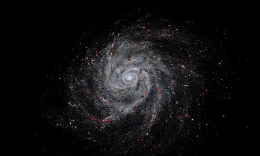
mode, in which scenes can be selected by an operator
or from a running script. This mode assists the user
during the journey in the virtual universe, by guiding
them towards the most interesting scenes. This mode
avoids the use of the hand-tracking system which can
sometimes require a time consuming and overwhelm-
ing training, but lets the visitor benefit from a full
immersive environment in which they can still roam.
This mode is especially designed to offer a quick ini-
tiation to a group of people.
   At the Solar System scale, time can be set arbitrar-
ily to focus, for example, on a specific planet config-
                                                              Figure 1: The International Space Station orbiting
uration, on a solar eclipse or on the peculiar position
                                                              above the earth. The Milky Way on the background
of a space probe or artificial satellite.
                                                              is reproduced by the Gaia data.
   The python scripting extension of VIRUP makes it
possible to manipulate most of the objects of the ren-
dering engine. This allows to fully script complex            NASA missions, extrapolated artistically if necessary.
sequences including transitions between them. This            7
                                                                 3D models of various bodies have also been ob-
feature has been used to create movies that can be            tained through the 3D Asteroid Catalogue8 .
displayed in 2D, 3D, 360◦ or 3D-VR-360◦ . A compan-              The data for the stars are taken from the Hippar-
ion video to the eBoss press release has been created         cos and/or the Gaia catalogue (Gaia EDR2), which
in 2020 4 . Recently, we produced a 21 minute long            contains 1.5 billion light sources. More than 4500 Ex-
documentary, The Archaeology of Light, a journey              oplanets are included via the Open Exoplanet Cata-
through the different scales of our Universe 5 .              log 9 , which aggregates various sources of exoplanet
                                                              data.
3      Overview of some viewable                                 The Milky Way is represented using a realis-
                                                              tic high-resolution simulation with initial conditions
       data sets                                              taken from the AGORA High-resolution Galaxy Sim-
                                                              ulations Comparison Project (Kim et al. 2016) and
Data visualized in VIRUP can be taken from both sim-          simulated with GEAR (Revaz & Jablonka 2012). Lo-
ulations and observations. For now, VIRUP has been            cal group dwarf galaxies are included through the
tested to visualize data from over 8 databases. Ex-           continuously-updated Local Group and Nearby Dwarf
tending the visualization with more data from other           Galaxies database of McConnachie (2012) 10 .
datasets is easy, thanks to the use of CSV, JSON and
                                                                 To represent the observed large scales of the Uni-
HDF5 formats as input to VIRUP and its tools.
                                                              verse, VIRUP includes the Sloan Digital Sky Survey
   At the Solar System scale, VIRUP includes both nat-
                                                              data (SDSS DR16) that consists of over 3.5 mil-
ural and artificial objects. Among them, a catalogue
                                                              lion objects (Ahumada et al. 2020). Simulated por-
of over 3000 satellites orbiting the Earth and other
                                                              tions of the Universe are taken either from the Eagle
spacecrafts, such as the Voyager and Pioneer probes.
                                                              project (Schaye et al. 2015), covering a volume of
The Solar System itself is rendered for a particular
date and time of day thanks to the data extracted       7 Full credits for artistic extrapolations are found in

from the tool of NASA JPL Horizons 6 . The ap- the sub-directories of : https://gitlab.com/Dexter9313/
pearance of the bodies is based on data from various prograde-data
                                                        8        Greg Frieger:https://3d-asteroids.space/
    4 https://www.youtube.com/watch?v=KJJXbcf8kxA               9 http://www.openexoplanetcatalogue.com/
    5 https://go.epfl.ch/ArchaeologyofLight                     10 http://www.astro.uvic.ca/ alan/Nearby_Dwarf_
                                                                                            ~
    6 https://ssd.jpl.nasa.gov/horizons.cgi                   Database.html

                                                          2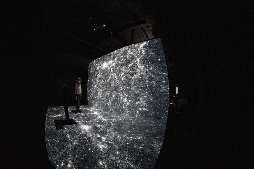
(100 Mpc/h)3 with 6.6 billion particles, or the Illus-
trisTNG project (Pillepich et al. 2018; Springel et al.
2018), with a volume of (205 Mpc/h)3 and 30 billion
particles.
Finally, VIRUP also contains the Cosmic Microwave
Background radiation map as observed by the Planck
Mission (Planck Collaboration et al. 2020) which is
used to illustrate the size of the observable Universe.
4 Multi-modal visualisation
systems
In addition to standard VR systems like gaming vir-
tual reality headsets, VIRUP also supports standard
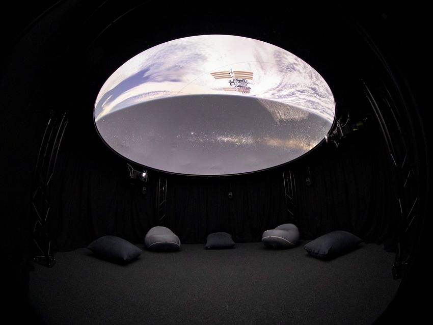
3D screens and has been adapted to run with more Figure 2: The Earth and International Space Station
advanced immersion systems, including 180◦ domes displayed by the Cupola at the eM+ laboratory
(2D or 3D), panoramic or CAVE projection screens,
which combine the images delivered by several pro- model of this installation. It also offers a major ben-
jectors. efit, ı.e. its open-viewing configuration, which allows
VIRUP has been tested so far on the following sys- for a much larger public to engage with the displayed
tems of the Laboratory for Experimental Museology content. The 0.5 CAVE uses stereo projection across
(eM+) 11 : the Cupola, 0.5 CAVE and Panorama+. the wall and floor, making it an ideal immersive space
for a wide range of contents.
The Cupola is a 5m diameter × 6m high visualisa-
tion system featuring two 3D beamers, whose images
are projected onto a hemispherical screen with an ef-
fective resolution of 4096 × 4096 pixels. The screen is
positioned above visitors, to allow for a unique view-
ing experience in a lying position. Since its concep-
tion in 2004, this visualisation system was featured
in multiple worldwide exhibitions, including Look Up
Mumbai (2015), Inside the Ethereal Eye (2016) and
Seven Sisters (2017), but also in miscellaneous in-
stallations at the UNSW Art & Design EPICentre
(2016-2019).
The 0.5 CAVE is a structural modification of the
original CAVE visualisation system. Instead of pro- Figure 3: The large scale structure of the Universe
jecting onto three walls and the floor, it displays im- from the IllustrisTNG simulations displayed by the
ages on a single wall and the floor, thanks to two 0.5 CAVE at the eM+ laboratory
2560 × 1600 3D beamers. One reason for this mod-
ification was the need to create a simplified touring
The Panorama+ is a 9m diameter × 3.6m high
11 https://www.epfl.ch/labs/emplus/ 360-degree stereoscopic system, also known as the
3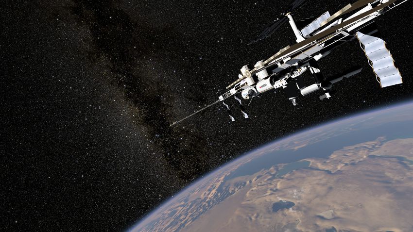
Advanced Visualisation and Interaction Environment              with single-precision variables, which are suited to
(AVIE). It has an effective resolution of 18000 × 2160          rendering on GPUs for performance reasons.
pixels, which is obtained by combining the images                 Finally, porting VIRUP towards the multi-projector
of a cluster of ten computers. Those images are then            systems described in Sec. 4 required to properly syn-
projected on the screen by five 3D beamers. This sys-           chronize several VIRUP instances running in parallel
tem makes it possible for visitors to explore wide vir-         on different computers.
tual environments, as well as large datasets. The first
AVIE was launched at UNSW in 2006 and since then,
multiple subsequent systems were deployed across the
                                                                5.1     Cosmological Large Scale struc-
world.                                                                  tures
                                                                5.1.1   Octree
                                                                As simulation datasets are often very large (several
                                                                billions of particles), they cannot be rendered at once
                                                                on standard GPUs at an acceptable frame rate re-
                                                                quired by VR systems. To solve this problem, data
                                                                must be split into chunks, in order to render only
                                                                what is currently seen by the user with an accept-
                                                                able level of detail. The technique we implemented
                                                                is greatly inspired from Szalay et al. (2008). We con-
                                                                struct a LOD-octree by splitting any node (portion
                                                                of the space) that contains more than 16’000 parti-
                                                                cles by 8. The octree generated is closer to a kd-tree
Figure 4:  The VIRUP sky displayed by the                       to ensure node balancing, i.e. we choose a splitting
Panorama+ at the eM+ laboratory                                 point along all three dimensions to ensure an equal
                                                                number of particles in each sub-node.
                                                                   During the rendering process, while walking the
                                                                tree, we use a rough approximate open angle crite-
5     Challenges and Algorithms                                 rion (taken as the diameter of the node divided by
                                                                its distance to the camera) to determine if recursion
The most important challenge faced when develop-                through a node is needed or not. A node that appears
ing VIRUP has been to load and render the large                 large on screen has to render its sub-nodes. On the
and varied datasets on the Graphics Processing Units            contrary, a node that appears small is rendered alone
(GPU), ensuring a frame rate of 90 images per sec-              without considering its sub-nodes (a node contains a
ond, essential to avoid sickness problems common in             sample of the content of its children nodes). A leaf
virtual reality environments and guarantee a fully              node will always be rendered if asked to do so, as it
immersive and smooth experience. A specific effort              has no children.
has been made to render several billions of points                 In order to determine what is physically large
contained in cosmological simulations. Ensuring a               enough to trigger a recursion, we could in princi-
smooth transition from one database to the next,                ple setup the opening criterion to a constant value
without freezing the system was essential.                      that would fit most situations well. However, be-
   Another challenge was to represent object over spa-          fore rendering, we have no information on the shape
cial scales spanning up to 27 orders of magnitude,              of the data to be displayed, on the region that will
from the meter, the typical scale of an artificial satel-       be observed by the user, nor on the type of hard-
lite, to about 100 Gly, the size of the observable Uni-         ware used. To avoid any surpise that could lead to a
verse. This is especially challenging when working              jerky rendering or a freeze-out, we developed a flex-

                                                            4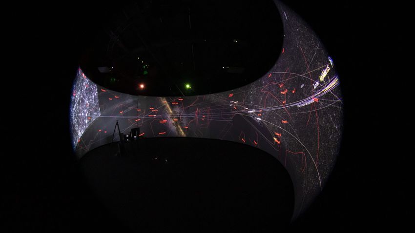
ible solution relying on the current frame rate. We           absorption, we first compute the luminance of the
use a PID-loop (proportional, integral, derivative) to        corresponding point. As dust is only absorbing (no
control the open angle criterion to maintain a given          emission), we simply need to march from the light
frame rendering time at any time. For a comfortable           source down to the camera once to get the absorption
VR experience it is set to 11 ms, i.e. 90 FPS.                coefficient and finally get the resulting luminance.
                                                              VIRUP also includes emissive media, as for example
octreegen To ensure the fastest possible loading of           the H-alpha emission of ionized gas. Those media
nodes, the octree is generated offline with a separate        are ray-marched from the boundary of their maps to
tool called octreegen 12 . The resulting octree is en-        the camera, including absorption, to obtain a total
coded in a specifically tailored file format which can        density value. We ray-march both emissive and ab-
be read by VIRUP as fast as possible. In particular,          sorbing media at the same time, so that the absorp-
the nodes data layout is already the same as the lay-         tion of emissive media is correctly computed along
out VIRUP passes to the graphics driver. The nodes            the depth.
can then be uploaded directly from the disk to the
GPU memory without further computation.

5.1.2   Reference frame and spacial scales
To account for the huge range of spatial scales cov-
ered by the data, up to 27 orders of magnitudes, while
using single-precision variables, we change the refer-
ence frame of the leaf node to which the camera is
the closest. Indeed, getting too close to a particu-
lar point will make it shake due to low precision of
the 32-bits floating-point variables (about 7 digits of
precision). When the camera enters a leaf node, all
of its 16’000 data points are moved to correspond to
                                                              Figure 5: The AGORA Milky Way-like galaxy simula-
coordinates of a reference frame which has its origin
                                                              tion displayed with a volumetric rendering including
to the closest point to the camera. When this closest
                                                              H−α emission and dust absorption.
point changes, the coordinates of all the data points
are re-computed to be centered on the new closest
point. This way, no matter how close to a point the
camera gets, the coordinates of the camera relative           5.1.4    Tone mapping
to this point will remain close to zero, which behaves
perfectly well in a floating-point representation.      The final state of VIRUP’s main framebuffer13 be-
                                                        fore post-processing is a luminance map in SI units.
                                                        There is a subtlety concerning the rendering of points
5.1.3 Volumetric rendering
                                                        that is worth developing here, as VIRUP renders a lot
To render dust and gas from a galaxy, as in our of point-based data. As points are objects without
Milky Way model for example, we compute 3D den- dimension, luminance is not defined. However, we
sity maps of the absorbing media from the simulated can associate to each points its illuminance which
snapshot. Those density maps will be loaded in GPU depends solely on its apparent magnitude obtained
memory and further used to perform ray-marching. from the luminosity of the object represented by the
   In our galaxies, we consider stars as light sources. point and its distance to the camera. This way, any
In order to properly render a star including dust
                                                               13 The buffer that contains the pixels resulting from all the
 12 https://gitlab.com/Dexter9313/octree-file-format/         main drawing commands.

                                                          5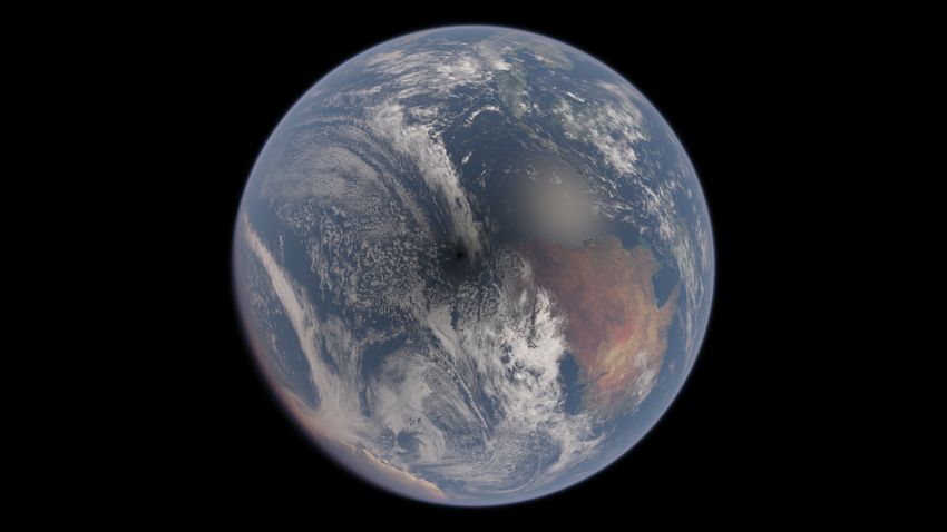
illuminance associated to a point, that is written in                  We added an optional auto-exposure function that
the framebuffer is converted to a luminance by sim-                 controls the exposure factor over time depending on
ply dividing it by the solid-angle of a pixel, ensuring             the scene average luminance, using a higher weight at
energy conservation.                                                the center of the scene. This function follows curves
    An important step of the post-processing is the                 of the adaptation properties of a typical human eye
conversion of the luminance to an RGB value which                   that were tailored to match those found in Dimitrov
will be displayed on the screen, a step also known                  et al. (2008).
as tone mapping. We tried to be as realistic as pos-                   To get the final tone mapping function, we multiply
sible matching what the human eye would see. To                     our scene luminance by the exposure factor before
this end, we use the concepts of dynamic range and                  passing it to our mapping function f which outputs
exposure.                                                           a normalized pixel value.
    The dynamic range is the factor between the                        For additional realism, we can also simulate the
dimmest visible luminance (lmin ) and the brightest                 fact that human eyes can no longer see colors be-
one (lmax ), without considering pixel saturation. To               low a certain luminance threshold. This is called the
roughly simulate a human eye, this factor must typ-                 Purkinje effect. We supplemented VIRUP with a simu-
ically be set to 100 000. We thus set lmin = 1 and                  lation of this effect, which gradually transforms RGB
lmax = 100 000. As typical LCD screens output pixel                 luminances below a certain threshold to grayscale.
values from 0 to 255 in integer values, we first need                  All these parameters : dynamic range, exposure
a function that maps the [1, lmax ] interval (1 being               and the toggleable Purkinje effect allow for a wide
                                          0.5
the dimmest visible luminance) to [ 255       , 1] (fragment        range of photo-realistic renderings. It is then possible
shaders output in the [0; 1] range, which is then multi-            to mimic either human eyes or photographic devices.
plied by 255). We use 0.5 as the smallest visible pixel             As an example, using a low dynamic range will mimic
value as it will be rounded to 1 by the discretization.             the rendering of an old spacecraft camera.
The mapping function also needs to be a logarith-
mic function if we want to see details at all scales,
especially in the dimmest regime.                                   5.2     Planetary systems
    We used the following mapping function that fulfill             5.2.1   Interpolation of Kepler Orbits
the previous requirements:
                                                                  To obtain the most accurate positions of the bodies of
               log (1 + (x − lmin )/c2 )                            the Solar System at a given time, we use data from
   f (x) =                                   (1 − c1 ) + c1
             log (1 + (lmax − lmin )/c2 )                           the NASA JPL Horizons tool. However, as VIRUP
                                                          (1)       is designed to be able to run offline, we cannot re-
              0.5
where c1 = 255     and c2 is a constant that defines the            trieve those positions from the NASA tool at launch
elbow of the logarithm in the range [lmin , lmax ] and is           time or when a new date is set. Instead, we rely on
set to about 1000. Note that the factor 255 can easily              a local database. For each celestial body, we have
be adapted to account for different screen dynamic                  downloaded its known orbital parameters at variable
ranges, useful for example for HDR ports.                           rates, daily for years close to 2021 (about 200 years
    The exposure is a factor that will ensure that the              before and after), weekly or more for the dates be-
dimmest visible luminance of the scene is mapped                    yond this time range. Note that this data does not
to 1 before being passed to our mapping function                    weight more than ten megabytes per body. To get
f . As a human eye can typically see in a range of                  the position of a body at any specific time, the corre-
luminance ranging from 10−6 to 108 cd/m2 , we can                   sponding orbital parameters are interpolated linearly
restrict the exposure factor to the range [1/(108 −                 between the two closest dates of our database that en-
lmax ), 1/10−6 ]. Here, 108 − lmax corresponds to the               compass this time. This is way more accurate than
dimmest visible luminance when the absolute visible                 linearly interpolating position-vectors, and gives re-
brightest luminance is 108 cd/m2 .                                  sults precise enough for most cases.

                                                                6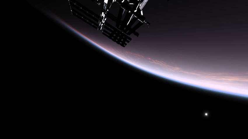
The proper treatment of the orbits of space probes
adds another difficulty. Indeed, they can strongly
modify their orbits on time scales much shorter than
one day, the smallest default time sampling of our
database. Such behaviour occurs typically when the
probe fired up its thrusters for example. We thus
detect such event and retrieve orbital parameters at
a much larger time resolution to ensure an optimal
interpolation.
   Peculiar cases exist when passing the ellipti-
cal/hyperbolic orbit transition. It happens when a
probe gets captured by a planet or when it achieves           Figure 6: Earth’s atmosphere as seen from the ISS
escape velocity for example. There, the interpola-            near sunset.
tion of the orbital parameters is no longer adequate
as the semi-major axis goes from minus infinity to
                                                              5.2.3   Celestial bodies light interaction
plus infinity or vice-versa. In such cases, to keep it
as accurate as possible, the orbit is determined by           Celestial bodies close to each other (mostly planet-
a non-linear interpolation of the state-vectors. This         moon systems or probes with other bodies) reflect
interpolation is however performed only during the            light from their star on each other. As the star is
shortest possible time interval.                              usually not a point-like source, they also cast smooth
                                                              shadows on each other. In computer graphics, a stan-
                                                              dard way to handle these subtle effects is to use global
                                                              illumination algorithms or shadow mapping. As most
                                                              of the time, celestial bodies can be approximated by
5.2.2   Atmospheres                                           spheres, we can use a much more efficient method.
                                                                 First, it is worth mentioning that while we take
Our atmospheres rendering is mostly based on                  into account light and/or shadows cast on probes by
Hillaire (2020). The main difference is that, as              planets or moons, we neglect the reverse, i.e., we ne-
VIRUP’s terrain rendering doesn’t account for ter-            glect light and/or shadows cast by probes on planets
rain height yet, we do not need to use their Aerial           or moons. When an object reflects light on another,
Perspective LookUp Table (LUT) or their Multiple              for example the Moon reflecting the Sun’s light on
Scattering LUT. Multiple scattering effects in at-            Earth, we consider the reflector to be a directional
mospheric rendering are mostly visible in terrain-            light source. We can compute the Moon’s phase as
induced shadows. As our planets still have some ellip-        seen from Earth to get the amount of light reflected
soidal terrain, aerial perspective effect must be taken       by the Moon and choose the Moon’s direction as
into account, however, there is no need to include a          the light source direction towards the Earth. Note
LUT with several layers. We split the atmospheric             that we do not perform multiple light bounces as we
rendering equation into two distinct parts : the in-          do not consider that some Moon light gets reflected
scattering (or emissive) part and the out-scattering          back from Earth to the Moon and so on. So, the
(or absorbing) part. Both components are stored in            Earth (resp. the Moon) reflects light from the Sun to
LUTs with similar parametrization as the Sky-View             the Moon (resp. the Earth) only once. A difficulty
LUT of Hillaire (2020). Those LUTs can be com-                appears however when moons are relatively close to
puted without terrain data while still taking terrain         their planet, as is Io to Jupiter, or the ISS to the
into account, as the terrain is described analytically        Earth for example. In these situations, we cannot
as an ellipsoid.                                              compute Earth’s phase and direction to infinity as

                                                          7
seen from the ISS, as the ISS would still receive light
from the planet as it would be way past sunset. In
these cases, we compute an approximation of a cor-
rected phase corresponding to the light receiver field
of view of the reflector and a corrected light direction
that points more or less towards the barycenter of the
light reflected by the reflector as seen by the receiver.
When an object casts a soft shadow on another, for
example when a solar eclipse occurs and the Moon
casts a shadow over Earth’s surface, we consider the
light source as a disks at infinity occluded by an-
other disk at infinity. As bodies can be ellipsoids, Figure 8: Solar eclipse that will occur on April 20th,
we first perform a transformation into a space where 2023. We can see the Moon’s soft shadow on the
the occluder is a sphere. This also transforms the south-west coast of Australia.
light source into this space. While this is incorrect, it
guarantee the shadow to have a correct shape. The
error induced by this approximation only affects the been supported by the Swiss National Science Foun-
smoothness of the shadow. dation under the AGORA Grant CRAGP2 178592.
In the particular case where both the light source It also received support from the EPFL Interdisci-
and the occluder are spheres, both will be seen as plinary Seed fund.
disk from any point on the shadow-receiver’s terrain
or on the atmosphere. We then simply compute the
ratio of light that still reaches this point to adjust its References
luminosity, which is a trivial geometric problem to
Ahumada, R., Prieto, C. A., Almeida, A., et al. 2020,
solve.
ApJS, 249, 3
Dimitrov, P. N., Guymer, R. H., Zele, A. J., An-
derson, A. J., & Vingrys, A. J. 2008, Investigative
ophthalmology & visual science, 49, 55
Hillaire, S. 2020, Computer Graphics Forum, 39, 13
Kim, J.-h., Agertz, O., Teyssier, R., et al. 2016, ApJ,
833, 202
McConnachie, A. W. 2012, The Astronomical Jour-
nal, 144, 4
Figure 7: The Moon during a new moon, lit mostly Pillepich, A., Springel, V., Nelson, D., et al. 2018,
by Earth’s reflection of sunlight. MNRAS, 473, 4077
Planck Collaboration, Aghanim, N., Akrami, Y.,
et al. 2020, A&A, 641, A1
Acknowledgements Revaz, Y. & Jablonka, P. 2012, A&A, 538, A82
We would like to thank Loı̈c Hausammann and Schaye, J., Crain, R. A., Bower, R. G., et al. 2015,
Mladen Ivkovic for very useful discussions. VIRUP has MNRAS, 446, 521
8Springel, V., Pakmor, R., Pillepich, A., et al. 2018,
MNRAS, 475, 676
Szalay, T., Springel, V., & Lemson, G. 2008, arXiv
e-prints, arXiv:0811.2055
9You can also read