A Comparison of Finite Control Set and Continuous Control Set Model Predictive Control Schemes for Model Parameter Mismatch in Three-Phase APF ...
←
→
Page content transcription
If your browser does not render page correctly, please read the page content below
ORIGINAL RESEARCH
                                                                                                                                          published: 02 August 2021
                                                                                                                                    doi: 10.3389/fenrg.2021.727364

                                           A Comparison of Finite Control Set and
                                           Continuous Control Set Model
                                           Predictive Control Schemes for Model
                                           Parameter Mismatch in
                                           Three-Phase APF
                                           Jianfeng Yang, Yang Liu * and Rui Yan
                                           School of Automation and Electrical Engineering, Lanzhou Jiaotong University, Lanzhou, China

                                           Model predictive control (MPC) methods are widely used in the power electronic control
                                           field, including finite control set model predictive control (FCS-MPC) and continuous
                                           control set model predictive control (CCS-MPC). The degree of parameter uncertainty
                                           influence on the two methods is the key to evaluate the feasibility of the two methods in
                                           power electronic application. This paper proposes a research method to analyze FCS-
                            Edited by:
                       Liansong Xiong,     MPC and CCS-MPC’s influence on the current prediction error of three-phase active
Nanjing Institute of Technology (NJIT),    power filter (APF) under parameter uncertainty. It compares the performance of the two
                                 China
                                           model predictive control methods under parameters uncertainty. In each sampling period
                         Reviewed by:
                              Hui Cao,
                                           of the prediction algorithm, different prediction error conditions will be produced when
        City University of Hong Kong,      FCS-MPC cycles the candidate vectors. Different pulse width modulation (PWM) results
                            SAR China
                                           will be produced when CCS-MPC solves the quadratic programming (QP) problem. This
                            Leilei Guo,
        Zhengzhou University of Light      paper presents the simulation results and discusses the influence of inaccurate modeling
                        Industry, China    of load resistance and inductance parameters on the control performance of the two MPC
                 *Correspondence:          algorithms, the influence of reference value and state value on prediction error is also
                            Yang Liu
                yang.lts@foxmail.com
                                           compared. The prediction error caused by resistance mismatch is lower than that caused
                                           by inductance mismatch, more errors are caused by underestimating inductance values
                   Specialty section:      than by overestimating inductance values. The CCS-MPC has a better control effect and
        This article was submitted to
                                           dynamic performance in parameter mismatch, and the influence of parameter mismatch is
        Process and Energy Systems
                          Engineering,     relatively tiny.
               a section of the journal
         Frontiers in Energy Research      Keywords: active power filter, model predictive control, power quality, finite control set- model predictive control,
                                           continuous control set model predictive control, error analyses
           Received: 18 June 2021
           Accepted: 16 July 2021
         Published: 02 August 2021
                                           INTRODUCTION
                             Citation:
   Yang J, Liu Y and Yan R (2021) A        In industry, daily life, and new energy power generation (Zhang et al., 2021), many electronic devices
Comparison of Finite Control Set and       are connected to the grid. These will cause harmonic pollution, consume reactive power and reduce
        Continuous Control Set Model
                                           the power quality of the power grid (Singh et al., 1999). Showing in Figure 1, The scale of China
Predictive Control Schemes for Model
        Parameter Mismatch in Three-
                                           power quality market caused by harmonic pollution is also expanding. In order to solve these power
                          Phase APF.       quality problems, many solutions are proposed, including improving the structure of converter
         Front. Energy Res. 9:727364.      topology (multilevel converter, Vienna rectifier, LCL) (Meynard and Foch, 1992; Kolar et al., 1996;
     doi: 10.3389/fenrg.2021.727364        Rodriguez et al., 2002), improving the control method (Rodriguez et al., 2013; Vazquez et al., 2017;

Frontiers in Energy Research | www.frontiersin.org                                1                                         August 2021 | Volume 9 | Article 727364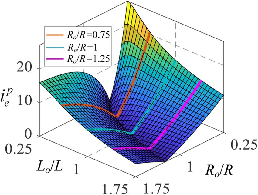
Yang et al.                                                                                       Error Comparison Between FCS-MPC and CCS-MPC

                                                                           carried out at each time cycle, so it is also called receding-horizon
                                                                           model predictive control.
                                                                              For a three-phase two-level converter, eight switch
                                                                           combination states can generate seven different vectors
                                                                           (including two zero vectors). That is, seven voltage outputs
                                                                           can be generated at each time. Therefore, the principle of
                                                                           FCS-MPC is necessary to:

                                                                           1) Establish the mathematical model of the converter (based on
                                                                              Kirchhoff’s law),
                                                                           2) The discrete prediction model is obtained,
                                                                           3) The cost function is established;
                                                                           4) FCS-MPC traverse seven vectors;
  FIGURE 1 | Market scale of power quality equipment in China.             5) The switch state combination is obtained under the minimum
                                                                              cost function, applied to the converter.

Zhou et al., 2021). With the increasing importance of power                   These predictive control methods inevitably produce
quality problem, APF was proposed. APF has become popular to               predictive error (PE) in practical application, PE affects the
improve power quality in the grid it can eliminate harmonics and           converter performance. Due to the nonlinear nature of FCS-
compensate for reactive power. APF detects harmonics based on              MPC, it is impossible to use the same mature analysis method as a
instantaneous reactive power theory and then injects harmonics             linear system to evaluate the influence of parameter changes
into the power grid through APF to achieve the purpose of                  (Bogado et al., 2014). Therefore, in previous studies, the influence
compensating harmonics (Garcia-Cerrada et al., 2007). Since                of model parameter mismatch has been empirically discussed by
APF was put forward, many control methods have appeared,                   studying models under different uncertainties (Kwak et al., 2014;
including proportional integral (PI) control, widely used in               Norambuena et al., 2019; Liu et al., 2020).
traditional industry (Garcia-Cerrada et al., 2007; Li et al.,                 Studies Liu et al. (2020) proposed that the MPC has the
2021). MPC is a control method developed from practice to                  problems of parameter mismatch (PM) and model
theory with the development of the industry. It has been widely            uncertainty, these problems can cause steady-state errors.
used in the field of power electronics and converters, which has a          Therefore, a new cost function is designed to improve the
good control performance (Marks and Green, 2002; Rodriguez                 robustness of FCS-MPC, that is, the integral error term is
et al., 2007; Bordons and Montero, 2015). The CCS-MPC                      added to the cost function, which effectively improves the
generates continuous output, and the optimal predictive value              robustness of conventional FCS-MPC. Previous work
is obtained by solving the constrained cost function (Bordons and          Norambuena et al. (2019) proposed a new design scheme,
Montero, 2015), but the modulation signal needs to be generated            which incorporated the past error into the new control system
by pulse width modulation (PWM). The FCS-MPC does not use                  action (as a new term of cost function), and adjusted the weight
PWM and depends on switching devices’ characteristics. In a                factors according to the past error, and improved the steady-state
limited set of switching vectors, the optimal vector is selected           performance under PM. To overcome the uncertainty of PM and
according to the tracking target and constraints (Aguilera et al.,         parameters, the studies in Kwak et al. (2014) proposed an
2013; Young et al., 2016). The general constrained MPC system              adaptive online parameter identification technology, which
performs many computations, and constrained CCS-MPC                        based on the least square estimation, the input current and
usually has a higher computing cost than FCS-MPC because                   input voltage are used to calculate the input inductance and
part or all of its optimization occurs online. When the condition is       resistance of active front end (AFE) in each sampling period
unconstrained, the analytical solution can be obtained to make             without additional sensors. Although the parameters are
the control off-line. The results’ solution needs to be obtained           uncertain, AFE still generates sinusoidal current with unit
through the optimization algorithm, which can solve the long-              factor (Ahmed et al., 2018). As in Young et al. (2016), the
term prediction problem. The FCS-MPC involves online                       inductance and resistance changes of FCS-MPC are analyzed
optimization in the next step or two. It does not require                  using the mathematical model in motor and inverter applications,
optimization algorithms with fast dynamic performance and is               respectively. In this paper, according to its application in APF, the
typically used in short-term prediction.                                   PE analysis is carried out using mathematical methods.
    CCS-MPC uses the plant’s dynamic mathematical model to                    Most previous research relies on empirical methods to study
predict, at the current time, which compares the predicted output          the control systems under the uncertainty of parameters in the
of from 1 to Np (prediction horizon) time stamp the with the               prediction model. This paper aims to analyze the prediction error
reference value. By establishing the cost function and solving the         under the condition of uncertain parameters, different states,
minimum problem, the optimal input of future Nc (control                   different reference, and load changes, the control performance of
horizon) can be obtained at each time stamp. In the converter              the two MPC methods on APF under the above conditions is
application, PWM modulation is needed, and the first group of               analyzed. that is, the compensation ability of APF to track
the control sequence is applied to the converter. Such a process is        harmonics. The analysis of prediction error is verified by

Frontiers in Energy Research | www.frontiersin.org                     2                                     August 2021 | Volume 9 | Article 727364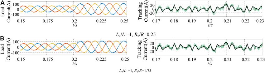
Yang et al.                                                                                           Error Comparison Between FCS-MPC and CCS-MPC

                                                                           FIGURE 4 | ip-iq method for harmonic detection.

                                                                             Three groups of switches Sx∈{Sa,Sb,Sc} are defined as two states:
  FIGURE 2 | Three-phase parallel APF structure diagram.                  on and off. In addition, dead zone protection is added to the
                                                                          output switch. These switches are defined as Eq. 1.

                                                                                              1;        if    S1 is ON and S4    is OFF
                                                                                       Sa
                                                                                              0;       if    S1 is OFF and S4     is ON
                                                                                              1;        if    S2 is ON and S5    is OFF
                                                                                       Sb                                                          (1)
                                                                                              0;       if    S2 is OFF and S5     is ON
                                                                                              1;        if   S3 is ON and S6     is OFF
                                                                                       Sc
                                                                                              0;       if    S3 is OFF and S6     is ON

                                                                             The vector composed of Sx in different switching states of
                                                                          three-phase two-level APF, by applying the complex Clark
                                                                          transformation 1–8 for eight possible switch configurations,
                                                                          the voltage vectors are be shown in Figure 3.

                                                                          Calculation of Harmonic Reference Current
                                                                          First of all, only when the standard harmonic current is
                                                                          detected, the APF can work normally, there are many
  FIGURE 3 | Two-level parallel APF switch vector in the complex          kinds of harmonic detection methods, at present, the most
  α-β frame.
                                                                          widely used method is the i p -i q method proposed by Akagi
                                                                          et al. (1984) and Xiong et al. (2020). Besides, PI is used to
                                                                          control the DC side capacitor voltage of APF, the
simulation. Finally, this paper gives the choice of control methods
                                                                          compensation part is injected to keep the energy
in different environments.
                                                                          interaction between the AC and DC sides and stabilize the
                                                                          voltage reference value (Xie et al., 2011). The principle is
                                                                          shown in Figure 4, it has good dynamic performance and
THREE-PHASE PARALLEL APF SYSTEM                                           tracking performance.
AND CURRENT CONTROL METHOD                                                    The detected three-phase harmonics iah, ibh and ich are taken as
                                                                          reference values where Xref  [iah;ibh;ich]. In the harmonic
The MPC relies on the APF mathematical model to predict how
                                                                          detection link, there is a period delay from current detection
the possible control actions affect its response. So, the action
                                                                          to harmonic calculation, so it cannot be used as the reference
expected to minimize a particular cost function is applied, and the
                                                                          value of the predicted value at the next moment. The reference
process is sequentially repeated. The appropriate model of APF is
                                                                          value can be predicted by Lagrange interpolation Eq. 2. In order
needed to obtain good control performance.
                                                                          to reduce the amount of computation, the low order interpolation
   Figure 2 shows the topology of the general voltage type APF,
                                                                          method is adopted in this paper
which can compensate the harmonic current generated by the
nonlinear load, where:                                                                           n
                                                                                                                  (n + 1)!
                                                                                iref (k + 1)   (−1)n−i                      · iref (k + i − n)     (2)
                                                                                                i0
                                                                                                               i!(n + 1 − i)!
1) ea, eb, ec are grid voltage,
2) ica, icb, icc are the output compensation current of APF,
3) iLa, iLb, iLc are load current, where L and R are the filter            Mathematical Model of Three-Phase APF
   inductance and equivalent resistance,                                  In the three-phase static coordinate system, assuming the three-
4) C is DC side capacitance, which stores energy for bidirectional        phase symmetry, according to Kirchhoff’s current law, the
   flow of APF, and grid energy, for Udc of the DC voltage, holds          dynamic Eq. 3 can be obtained, where uca,ucb, and ucc are the
   stability.                                                             output voltage of APF.

Frontiers in Energy Research | www.frontiersin.org                    3                                           August 2021 | Volume 9 | Article 727364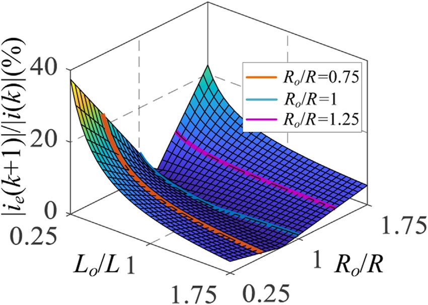
Yang et al. Error Comparison Between FCS-MPC and CCS-MPC
objective and constraint problems, and through PWM
modulation, achieve fixed switching frequency.
According to Eq. 3, let the state variable be x [iα; iβ], input is
u [eα-ucα; eβ-ucβ], therefore, the state-space model of three-
phase two-level APF in α-β coordinate can be obtained:
x_ Ax + Bu
(9)
y Cx
R 1
⎢
⎡
⎢ − 0 ⎤⎥⎥ ⎢
⎡ ⎤⎥⎥⎥
FIGURE 5 | FCS-MPC principal diagram. ⎢
⎢
A⎢
⎢
L ⎥⎥⎥⎥, B ⎢ ⎢
⎢
⎢
⎢
L ⎥⎥⎥, C 1
⎢ ⎥⎥⎦ ⎢
⎢ ⎥ (10)
⎢
⎣ R ⎣ 1 ⎥⎦ 1
0 −
L L
⎪
⎧
⎪
dia
ea − Ria − uca
⎪
⎪ L The continuous system (Eq. 9) is discretized:
⎪
⎪ dt
⎪
⎪
⎨ dib x(k + 1) Gx(k) + Fu(k)
⎪ L eb − Rib − ucb (3) (11)
⎪
⎪ dt y(k) Cx(k)
⎪
⎪
⎪
⎪ G eATs , F eATs − IA−1 B
⎪ L dic e − Ri − u
⎩ (12)
c c cc
dt
The Euclidean norm produces an over proportional cost (in
Equation 4 can be obtained by discretizing a-phase in Eq. 3: powers of two) compared to the 1-norm, giving a higher
R Ts penalization of more considerable errors than smaller ones. It
ip (k + 1) 1 − Ts i(k) + (e(k) − uc (k)) (4) can be used to control variables closer to the reference and reduce
L L
the ripple amplitude. First, the prediction horizon is set as Np, the
control horizon is set as Nc, and the weight factor of each state
Traditional FCS-MPC quantity is Qe. Simultaneously, to hope that the control action is
The principle of FCS-MPC is shown in Figure 5 (Aguirre et al., not too large, the constraint on the control quantity is added, and
2018). the weight factor is R. Through proof in the Supplementary
In FCS-MPC, 8 switch vectors shown in Figure 3 are cycled in Appendix, it can establish the cost function Eq. 13.
turn, these 8 states represent the 8 outputs of APF, which are Np
substituted into the mathematical model to predict the output at 2
J(k) iref (k + i|t) − ip (k + i|t)
the next moment. Therefore, parameter matching is particularly Qe
i1
(13)
important. Tracking harmonics in a three-phase coordinate Nc
system will produce the accumulated error, in order to better + u(k + i − 1|t)2R
i1
follow the detected harmonics, cost function is established in the
α-β coordinate system, shown in Eq. 5. The minimum switching One of the essential characteristics of MPC is that it can
state of the cost function is solved, APF is controlled by consider the constraints in the optimization process. When APF
modulation signals generated by FCS-MPC (Aguirre et al., 2018). works, it does not violate the system characteristics, so the cost
function is transformed into a constrained quadratic
J iref (k + 1) − ip (k + 1) + hlim (i) + ci s2 (i) (5)
Q programming (QP) problem.
α (k
iref + 1) ipα (k + 1)
iref (k + 1) , i (k + 1) + 1)
p (6) 1 T
ref
iβ (k + 1) p iβ (k min U HU + f T U
U 2
λα 0 s.t. U min ≤ U(k) ≤ U max (14)
Q (7)
0 λβ
Y min ≤ Y(k) ≤ Y max i 1, 2, ..., n, ..., p
Q is the coefficient of the tracking harmonic reference in the a-β
coordinate system, hlim is the limiting amplitude of predicted
output value, such as Eq. 8, s is the number of switch changes in
the period, and ci is its weighting factor.
0, if ip (k + 1) ≤ imax
hlim (i) (8)
∞, if ip (k + 1) > imax
Traditional CCS-MPC
As shown in Figure 6, the principle of CCS-MPC is to solve the
optimization problem and apply the optimal control input to the
FIGURE 6 | CCS-MPC principal diagram.
system. The most significant advantage is considering the multi-
Frontiers in Energy Research | www.frontiersin.org 4 August 2021 | Volume 9 | Article 727364Yang et al. Error Comparison Between FCS-MPC and CCS-MPC
The above minimization problem is equivalent to solve a
convex quadratic programming problem, in this paper, the
interior point method is used to solve quadratic programming
problems. The algorithm’s purpose is to find a feasible descent
direction from the interior point in a feasible region so that the
interior point moves along this direction, reducing the value of
the cost function. The interior point method is practical and has
low complexity, which is one of the core algorithms to solve the
QP problem.
PE IN MPC DUE TO MODEL PM
Manufacture, service, and life of converter, these will inevitably
affect the control effect because of the parameter error. In the PE
analysis of FCS-MPC, this paper adopts the same analysis method
as Young et al. (2016). In the parameter estimation and sensitivity FIGURE 7 | The PE in FCS-MPC.
analysis, the assumption that load and load parameters change
simultaneously is balanced.
Meanwhile, to analyze the effectiveness of CCS-MPC control seven predictive output switching states of FCS-MPC. In this
performance for actual parameter mismatch or disturbance, the paper, the control variable method is used to take the switching
inductance and resistance analysis in Young et al. (2016) is also state of a particular combination. For the convenience of analysis,
used to analyze the load resistance value R and load inductance the output is assumed to be a zero-vector. The PE caused by
value L, the impact of their changes on prediction error. Different current and APF output voltage has been discussed in Young et al.
disturbances are added to the load resistance, and inductance, (2016). under the parameter (Ts 0.0001, R 2 W, L 2 mH), as
Ro R + Rd, Lo L + Ld, R and L are the actual parameters, Rd and shown in Figure 7, the sensitivity of the absolute error value is
Ld are the disturbances. determined when the resistance value and inductance value do
not match. It can be found that the inductance value mismatch
PE in FCS-MPC has a more significant influence on the absolute value of the
In FCS-MPC, the output prediction value under PM will predicted current error than the mismatch of the resistance value;
affect the judgment of cost function, which will lead to a non- When parameters match, |ie| 0; When the resistance value is
optimal switch vector state is selected, thus affecting the underestimated, it has more influence on PE than when it is
actual control effect. In this paper, after adding the mismatch overestimated. Besides, we can find that the error caused by
factors, R o R + R d , R o R + R d , the new prediction method overestimation of inductance is smaller than that caused by
is Young et al. (2016), underestimation, and the distribution is asymmetric.
ip (k + 1) 1 − Ts Ro i(k) + Ts (e(k) − uc (k)) (15) PE in CCS-MPC
Lo Lo This section is compared with FCS-MPC, CCS-MPC does not
need to establish a particular cost function, its constraints and
ip (k+1) is the prediction value of the next time after the Euler
control objectives are included in its cost function, but the control
difference, and Ts is sample time. In this paper, a one-step
of APF needs PWM modulation first. In CCS-MPC, U is obtained
prediction is used. To analyze the prediction error value under
by solving the cost function, and APF is controlled to compensate
the influence, we have this definition:
for the harmonic current of the power grid. The solution of U is
ie ip − ip (16) based on the solution of the QP problem, so the change of
parameters will affect the discrete state-space model and the
Substituting (Eqs 3, 15) into (Eq. 16), ie can be obtained: predicted value for the future. In calculating ip (k + Np) iteratively,
[(Rd L − RLd )i(k) + Ld (e(k) − u(k))]Ts errors will accumulate, which will eventually affect the result, and
ipe (17) may not be the optimal modulation voltage. In order to analyze
L(L + Ld )
the influence of parameter mismatch on the control effect of CCS-
The prediction error can be calculated by Eq. 17. It can be MPC, a state space model with disturbance is established:
found Eq. 17 that the error value depends not only on the
x(k) + Fu(k)
x(k + 1) G
resistance and inductance value but also on the current i(k),
the grid voltage e(k), and the output value u(k) of APF. It is worth y(k) Cx(k) (18)
noting that if there is an error in the current prediction, it will where
accumulate to the next time. In a small sampling period, the grid
voltage e(k) remains unchanged, and u(k) depends on one of the eATs , F eATs − I A
G −1 B
(19)
Frontiers in Energy Research | www.frontiersin.org 5 August 2021 | Volume 9 | Article 727364Yang et al. Error Comparison Between FCS-MPC and CCS-MPC
obtained in this paper should be substituted into the APF
mathematical model. Meaning, the compensated grid current
value at the next moment and the error value is defined as:
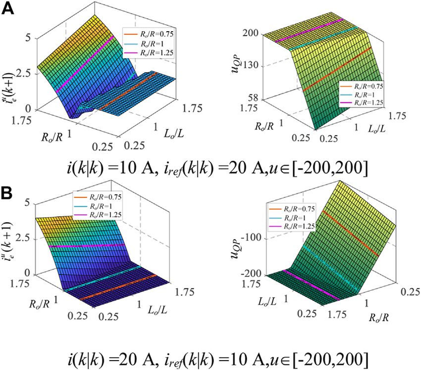
iue (k + 1) i(k + 1|k) − i(k + 1|k) (23)
After the PM is introduced, the QP problem is solved
respectively, and the relationship in Figure 8 can be obtained
with mismatched inductance and resistance values.
uQP is the first group of solved control sequences, that is, the
input applied to APF. CCS-MPC and FCS-MPC have the same
characteristics of asymmetric distribution of resistance and
inductance sensitivity, because CCS-MPC can deal with
multiple constraints, it will also have a certain impact on the
error. This paper analyzes the error under different conditions.
In different reference and state, when the parameters do not
match, we will establish different state matrix and input matrix by
substituting different inductance and resistance values. Through
FIGURE 8 | The terminal PE in CCS-MPC.
the Supplementary Appendix to solve the control sequence, the
first group of control sequence is applied to the discrete state
space equation, and their next time prediction values are
Ro Rd + R obtained, respectively. By subtracting them, we get the
⎡⎢⎢⎢ −L ⎥⎥⎥ ⎢
0 ⎥⎤⎥ ⎡ ⎢
⎢
−
Ld + L
0 ⎤⎥⎥⎥ prediction error in Figure 9:
⎢⎢⎢⎢ o
A ⎥⎥ ⎢
⎢
⎢
⎢
⎢
⎥⎥⎥
⎥⎥ (20)
⎢⎢⎣ Ro ⎥⎥⎦ ⎢ ⎢
⎣ Rd + R ⎥⎥⎦
0 − 0 − 1) Compared with the terminal error in Figure 8, PE value is
Lo Ld + L smaller, because it is solved in the entire prediction horizon.
1 2) There is a correlation between PE and input, when the input
⎢
⎡
⎢
⎢ Ld + L
0 ⎤⎥⎥
⎥⎥⎥
⎢ ⎢ reaches the limit, PE will increase significantly.
B ⎢
⎢
⎢ ⎥⎥⎥ (21)
⎢
⎢
⎣ 1 ⎥⎥⎦ 3) When the input is in the limited range, PE can keep a specific
0 constant value.
Ld + L
4) It should be noted that when the state value is different, the
After the state matrix changes, the error value is obtained by influence caused by resistance and inductance will also
Supplementary Appendix. change.
ipe ip k + Np |t − ip k + Np |t (22)
Let the prediction horizon Np 10 and the control horizon
Nc 4, for the convenience of analysis, set the initial current
value i (k|k) 20 A, u (k) 100 in the control horizon. Figure 8
shows the PE value by the terminal when the resistance and
inductance values do not match. In other words, this error is the
result of increasing at the time stamp k + p with the prediction
horizon, it is shown in the Supplementary Appendix.
Different from FCS-MPC, because of the characteristic of
CCS-MPC, the error is superposition, the influence of load
error on the error is also different. when Ro/R 1, Lo/L 1,
the PE 0; When Ro/R < 1 and Lo/L < 1, the PE is more sensitive
and has a more significant impact on the results; compared with
the change of resistance, the change of inductance has more PE;
When Ro/R > 1 and Lo/L > 1, the error value has a lower influence
on the prediction results and has asymmetry. Therefore, in
practice, when the load parameters are overestimated or
underestimated in the mathematical model, especially the
inductance value, the control effect will be greatly affected.
CCS-MPC of APF needs to solve the QP problem, The first
group of control sequences is applied to APF after PWM is
applied. To compare the PE value of the grid current after the
FIGURE 9 | The PE and first group control value in CCS-MPC.
output of PM with APF, the first group of control sequences u is
Frontiers in Energy Research | www.frontiersin.org 6 August 2021 | Volume 9 | Article 727364Yang et al. Error Comparison Between FCS-MPC and CCS-MPC
1) The closer the reference value is to the value of state, the
smaller the PE is, and near it, the PE is close to zero.
2) When the resistance value is constant and Lo/L < 1, the change
of PE is more sensitive than the inductance value is
overestimated. If Lo/L 1, PE is equal to zero.
3) When Lo/L 1, The change of PE is affected by the
mismatching of resistance parameters. PE increases near
the iref (k|k) 0.
4) The larger the gap between the state value and the reference
value, the larger the PE.
For CCS-MPC, the cost function contains the reference value
in the whole prediction horizon, so the reference value will affect
the generation of control sequence and cause prediction error,
which will be found in the Supplementary Appendix. Figure 11
shows that when the reference variables remain unchanged, the
FIGURE 10 | Steady-state performance change with reference change.
5) The results of CCS-MPC are mainly affected by the change of
resistance value, which is related to the coefficient of input
matrix R.
Steady State Performance Under State
Value and Reference Value Change
This section focuses on the influence of PM on prediction error
and control effect under different reference values and current
state values. In this section, the control variable method is used to
analyze the influence of Ro/R and Lo/L on PE, the possible result
when the state value or the reference value changes. The
performance of FCS-MPC has been analyzed in Young et al.
(2016). This section mainly analyzes the steady-state
performance of CCS-MPC.
In Figure 10, it is different from the published work, we
analyzed the sensitivity of parameter mismatch when the state
value changes, as in Figure 9, we set the parameters and reference
values to be variation, and the changes of inductance value and
FIGURE 11 | Steady-state Performance change with state change.
resistance value are discussed respectively:
Frontiers in Energy Research | www.frontiersin.org 7 August 2021 | Volume 9 | Article 727364Yang et al. Error Comparison Between FCS-MPC and CCS-MPC
TABLE 1 | Simulation model parameters. and (D) describes the THD of the distorted load current. At
Parameter Value 0.17 s, THD is 16.48%, and the main harmonic is the 5th, 7th,
11th, 13th, 17th, and 19th harmonics.
Grid voltage and f 380 V, 50 Hz
DC voltage 800 V
DC capacitor C 4,000 μF Steady State and Dynamic State
Inductor
Resistor
2 mH
0.01 Ω
Performance Under Change of Inductance
Load Resistor 8 Ω Value
Ts 1 × 10⁻⁴ s Figure 13 shows the load and reference currents after harmonic
compensation with FCS-MPC when Ro/R 1 and Lo/L are 0.25, 1,
and 1.75, respectively. (A): The results show that PM will increase
influence of the change of reference value on PE is analyzed, and the steady-state error of FCS-MPC when the inductance is
the changes of inductance value and resistance value are discussed seriously underestimated, the current waveform is worse than
respectively: (B,C). The follow-up of the harmonic reference value is also poor,
confirming the above analyzes on PE when the inductance value
1) PE is small when the state value is close to the reference value. is underestimated. (B) describes the case of no error in inductance
2) When the Ro/R 1 and Lo/L < 1, the change of PE is more and resistance values, the effect of three-phase compensation is
sensitive than when the value is overestimated; If Lo/L 1, PE improved, and it also has good follow-up when the load changes
is equal to 0. suddenly. In (C), the inductance value is overestimated, so the
3) When Lo/L 1, PE increases rapidly with the underestimation compensated current waveform is close to (B), and the control
of resistance. PE increases near the i (k|k) 0. effect is slightly worse than (B).
4) The larger the difference between the reference value and the Figure 14 shows the load and reference currents after
state value, the larger PE. harmonic compensation with CCS-MPC when Ro/R 1 and
Lo/L are 0.25, 1, and 1.75, respectively. Under the same
conditions, the control effect of CCS-MPC is better than that
SIMULATION RESULTS AND ANALYSIS of FSC-MPC. When the inductance is underestimated, steady-
state error (SSE) is smaller than that of FCS-MPC; The dynamic
In this section, simulation results verify the performance of CCS- performance improves attributed to CCS-MPC controlling in the
MPC and FCS-MPC on PM, the MATLAB/Simulink model is multiple time horizon in the future. However, from the following
established, and their results are compared. The simulation effect, in (A), the dynamic effect is worse than (C), verifying that
parameters are shown in Table 1. when the resistance value is underestimated, the influence on the
control effect is greater; At the same time, it can be found that the
Performance of APF performance is the best when parameter matching does
According to the above parameters, in the APF system, the load not occur.
adopts a three-phase uncontrollable rectifier circuit to verify the
above analysis results in SIMULINK. The dynamic performance
of predictive control abruptly changes the load value from 8 to
Steady State and Dynamic State
4 Ω in 0.2 s, verifying the dynamic performance of predictive Performance Under Change of Resistance
control. As shown in Figure 12, (A) describes the three-phase Value
voltage of the APF system, and (B) describes the uncompensated Figure 15 shows the load current and reference current following
three-phase load current. Due to the influence of nonlinear load, harmonic compensation with FCS-MPC when Lo/L 1 and Ro/R
the load current is distorted, (C) is the three-phase harmonics are 0.25, 1, and 1.75. Compared with Figure 14, in the same case,
detected by Section Calculation of Harmonic Reference Current, When the resistance value is underestimated, the effect on the
FIGURE 12 | Performance of APF under nonlinear load.
Frontiers in Energy Research | www.frontiersin.org 8 August 2021 | Volume 9 | Article 727364Yang et al. Error Comparison Between FCS-MPC and CCS-MPC
FIGURE 13 | Transient response with FCS-MPC under load inductance modeling error.
FIGURE 14 | Transient response with CCS-MPC under load inductance modeling error.
steady state error is not as great as when the inductance value is increase the objective function. In CCS-MPC, the dynamic
underestimated. Compared with (A,B), the steady-state error performance is slightly worse when the resistance is
caused by the mismatch of the resistance value is larger, but it overestimated, this result is consistent with the analysis in the
smaller than that caused by the mismatch of inductance value. previous section.
FCS-MPC has no modulation control, the switching frequency
Changes of THD During PM varies according to load conditions, they are difficult to compare
Figure 16 shows the load and reference currents after harmonic fairly. In order to make a fair simulation comparison, the THD of
compensation with CCS-MPC when Lo/L 1 and Ro/R are 0.25, the two methods is consistent when the load does not change.
1, and 1.75, respectively. Compared with Figure 15, under the As shown in Figure 17, in order to better compare the
same conditions, its dynamic performance is better when the performance between two control methods, the THD
parameters do not match. However, when a large gap occurs harmonic compensation results under different mismatches
between the reference value and the state value, it may still cause a degrees are analyzed, which are consistent with the above
large tracking error, the reason is that the gap between them will analysis results.
Frontiers in Energy Research | www.frontiersin.org 9 August 2021 | Volume 9 | Article 727364Yang et al. Error Comparison Between FCS-MPC and CCS-MPC
FIGURE 15 | Transient response with FCS-MPC under load resistance modeling error.
FIGURE 16 | Transient response with CCS-MPC under load resistance modeling error.
5) In general, CCS-MPC has high fault tolerance when parameters
and load are easy to change with the environment, and FCS-MPC
has better performance under stable conditions.
Significantly, the actual control effect is affected by other
conditions. Although CCS-MPC has good performance when
the PM and the load change, and it can add constraints to the
system input and state, the actual control effect is also affected by
other control parameters, such as prediction horizon Np, horizon
Nc, state; input constraints, and weight factors, it is not easy to get
the optimal parameters among these factors. In addition, it
FIGURE 17 | Changes of THD with two methods. should be noted that the factor of the weight matrix can also
be changed to reduce the error accumulation in the future time
horizon. FCS-MPC shows good performance in a stable
1) Lo/L Ro/R 0.25, that is, when the resistance is underestimated, condition, which also has a great relationship with the
FCS-MPC causes the more significant error because of in a short processor performance and sampling time Ts, moreover, it can
time domain, the results cannot be optimized. The THD with also improve the control effect by multi-step prediction or
FCS-MPC also decreases with the decreases of load. optimizing the cost function. For the application of predictive
2) We can see from Figure 16 that the dynamic performance of current control in converter field, according to the above analysis,
CCS-MPC is obviously better. the value of the load current will affect the control effect.
3) When the parameters are underestimated, the error caused by Secondly, the reference value and the current state value will
CCS-MPC is smaller than that caused by FCS-MPC. also significantly impact the control effect. At different levels of
4) After stabilization, the steady-state performance of FCS-MPC the power grid, the two methods may have different control
is better, which is related to its short time horizon control. effects, which can be further analyzed in the future.
Frontiers in Energy Research | www.frontiersin.org 10 August 2021 | Volume 9 | Article 727364Yang et al. Error Comparison Between FCS-MPC and CCS-MPC
CONCLUSION persuasion of this paper limited. As for the comparison of
CCS-MPC and FCS-MPC in design and experiment, some
This paper focuses on the two popular MPC methods of three- simulations or experiments given in the published papers can
phase APF, FCS-MPC, and CCS-MPC, and analyzes their provide some reference for readers (Aguilera et al., 2013; Bordons
inductance and resistance values when they are not matched. and Montero, 2015; Young et al., 2016; Ahmed et al., 2018;
And then analyzes the influence of the current state and harmonic Wendel et al., 2018; Karamanakos and Geyer, 2019).
reference value. The analysis and results show that for the two
control methods, the error caused by underestimating inductance
value is greater than that caused by overestimating, and the DATA AVAILABILITY STATEMENT
control effect is also significantly affected. Compared with
inductance mismatch, the error caused by resistance mismatch The raw data supporting the conclusion of this article will be
is smaller and approximately symmetrical. Regarding the made available by the authors, without undue reservation.
influence on the results, the mismatch of inductors is
dominant, so more accurate inductance values are needed in
the actual industrial environment. The analysis in Section Steady AUTHOR CONTRIBUTIONS
State and Dynamic State Performance Under Change of
Inductance Value also relates to the power grid level and the Conceptualization and formal analysis, RY; investigation, YL;
nonlinear load size, different reference values and state values will resources and supervision, JY; validation and writing—original
have a particular impact on the prediction results. Finally, the draft preparation, YL; writing—review and editing, YL. All
control method also needs to consider the load fluctuation. authors have read and agreed to the published version of the
After the analysis in this paper, the results show that CCS- manuscript.
MPC has a better control effect and dynamic performance, and
the influence of PM is relatively tiny. But when the system is
stable, THD is lower with FCS-MPC. In different situations, the FUNDING
selection of different MPC methods can improve the performance
of APF, and the asymmetry of load parameter changes can help Project supported by National Natural Science Foundation of
determine which MPC method APF should use in different China (NSFC) (61863023).
situations. In published studies, parameter identification and
observer setting are effective solutions, they can effectively
improve the sensitivity of MPC in parameter changes. In the SUPPLEMENTARY MATERIAL
future, the discussion at the end of the fourth section, which is
worthy of attention in the following research. The Supplementary Material for this article can be found online at:
Detailed simulation results are provided in this paper. https://www.frontiersin.org/articles/10.3389/fenrg.2021.727364/
However, the lack of experimental research makes the full#supplementary-material
Garcia-Cerrada, A., Pinzon-Ardila, O., Feliu-Batlle, V., Roncero-Sanchez, P., and
REFERENCES Garcia-Gonzalez, P. (2007). Application of a Repetitive Controller for a Three-
phase Active Power Filter. IEEE Trans. Power Electron. 22 (1), 237–246.
Aguilera, R. P., Lezana, P., and Quevedo, D. E. (2013). Finite-Control-Set Model doi:10.1109/TPEL.2006.886609
Predictive Control with Improved Steady-State Performance. IEEE Trans. Ind. Karamanakos, P., and Geyer, T. (2019). Guidelines for the Design of Finite Control
Inf. 9 (2), 658–667. doi:10.1109/TII.2012.2211027 Set Model Predictive Controllers[J]. IEEE Trans. Power Electron. 35 (7),
Aguirre, M., Kouro, S., Rojas, C. A., Rodriguez, J., and Leon, J. I. (2018). Switching 7434–7450. doi:10.1109/TPEL.2019.2954357
Frequency Regulation for FCS-MPC Based on a Period Control Approach. Kolar, J. W., Ertl, H., and Zach, F. C. (1996). “Design and Experimental
IEEE Trans. Ind. Electron. 65, 5764–5773. doi:10.1109/tie.2017.2777385 Investigation of a Three-phase High Power Density High Efficiency unity
Ahmed, A. A., Koh, B. K., and Lee, Y. I. (2018). A Comparison of Finite Control Set Power Factor PWM (VIENNA) Rectifier Employing a Novel Integrated Power
and Continuous Control Set Model Predictive Control Schemes for Speed Semiconductor Module,” in Proceedings of Applied Power Electronics
Control of Induction Motors. IEEE Trans. Ind. Inf. 14 (4), 1334–1346. Conference APEC ’96, San Jose, CA, USA, 2, 514–523. doi:10.1109/
doi:10.1109/TII.2017.2758393 APEC.1996.500491
Akagi, H., Kanazawa, Y., and Nabae, A. (1984). Instantaneous Reactive Power Kwak, S., Moon, U.-C., and Park, J.-C. (2014). Predictive-Control-Based Direct
Compensators Comprising Switching Devices without Energy Storage Power Control with an Adaptive Parameter Identification Technique for
Components. IEEE Trans. Ind. Applicat. IA-20 (3), 625–630. doi:10.1109/ Improved AFE Performance. IEEE Trans. Power Electron. 29 (11),
TIA.1984.4504460 6178–6187. Nov. 2014. doi:10.1109/TPEL.2014.2298041
Bogado, B., Barrero, F., Arahal, M. R., and Toral, S. L. (2014). “Sensitivity to Li, H., Liu, Y., Qi, R., and Ding, Y. (2021). A Novel Multi-Vector Model Predictive
Electrical Parameter Variations of Predictive Current Control in Multiphase Current Control of Three-phase Active Power Filter. Ejee 23 (1), 71–78.
Drives[C]// Industrial Electronics Society,” in IECON 2013 - 39th Annual doi:10.18280/ejee.230109
Conference of the IEEE (IEEE). Liu, X., Zhou, L., Wang, J., Gao, X., Li, Z., and Zhang, Z. (2020). Robust Predictive
Bordons, C., and Montero, C. (2015). Basic Principles of MPC for Power Current Control of Permanent-Magnet Synchronous Motors with Newly
Converters: Bridging the Gap between Theory and Practice. EEE Ind. Designed Cost Function. IEEE Trans. Power Electron. 35 (10), 10778–10788.
Electron. Mag. 9 (3), 31–43. doi:10.1109/MIE.2014.2356600 doi:10.1109/TPEL.2020.2980930
Frontiers in Energy Research | www.frontiersin.org 11 August 2021 | Volume 9 | Article 727364Yang et al. Error Comparison Between FCS-MPC and CCS-MPC Marks, J. H., and Green, T. C. (2002). Predictive Transient-Following Control of Xiong, L., Liu, X., Zhao, C., and Zhuo, F. (2020). A Fast and Robust Real-Time Shunt and Series Active Power Filters. IEEE Trans. Power Electron. 17 (4), Detection Algorithm of Decaying DC Transient and Harmonic Components in 574–584. doi:10.1109/TPEL.2002.800970 Three-phase Systems. IEEE Trans. Power Electron. 35 (4), 3332–3336. Meynard, T. A., and Foch, H. (1992). “Multi-level Conversion: High Voltage doi:10.1109/tpel.2019.2940891 Choppers and Voltage-Source Inverters,” in PESC ’92 Record. 23rd Annual Young, H. A., Perez, M. A., and Rodriguez, J. (2016). Analysis of Finite-Control-Set IEEE Power Electronics Specialists Conference, Toledo, Spain, 1, 397–403. Model Predictive Current Control with Model Parameter Mismatch in a Three- doi:10.1109/PESC.1992.254717 phase Inverter. IEEE Trans. Ind. Electron. 63 (5), 3100–3107. doi:10.1109/ Norambuena, M., Lezana, P., and Rodriguez, J. (2019). A Method to Eliminate Steady- TIE.2016.2515072 State Error of Model Predictive Control in Power Electronics. IEEE J. Emerg. Sel. Top. Zhang, K., Zhou, B., Or, S. W., Li, C., Chung, C. Y., and Voropai, N. I. (2021). Power Electron. 7 (4), 2525–2530. doi:10.1109/JESTPE.2019.2894993 Optimal Coordinated Control of Multi-Renewable-To-Hydrogen Production Rodriguez, J., Lai, J-S., and Peng, F. Z. (2002). Multilevel Inverters: a Survey of System for Hydrogen Fueling Stations. IEEE Trans. Ind. Applicat. (99), 1–1. Topologies, Controls, and Applications. IEEE Trans. Ind. Electron. 49 (4), doi:10.1109/TIA.2021.3093841 724–738. doi:10.1109/TIE.2002.801052 Zhou, B., Zhang, K., Chan, K. W., Li, C., Lu, X., Bu, S., et al. (2021). Optimal Rodriguez, J., Pontt, J., Silva, C. A., Correa, P., Lezana, P., Cortes, P., et al. (2007). Coordination of Electric Vehicles for Virtual Power Plants with Dynamic Predictive Current Control of a Voltage Source Inverter. IEEE Trans. Ind. Communication Spectrum Allocation. IEEE Trans. Ind. Inf. 17 (1), 450–462. Electron. 54 (1), 495–503. doi:10.1109/tie.2006.888802 doi:10.1109/tii.2020.2986883 Rodriguez, J., Kazmierkowski, M. P., Espinoza, J. R., Zanchetta, P., Abu-Rub, H., Young, H. A., et al. (2013). State of the Art of Finite Control Set Model Conflict of Interest: The authors declare that the research was conducted in the Predictive Control in Power Electronics. IEEE Trans. Ind. Inf. 9 (2), 1003–1016. absence of any commercial or financial relationships that could be construed as a doi:10.1109/tii.2012.2221469 potential conflict of interest. Singh, B., Al-Haddad, K., and Chandra, A. (1999). A Review of Active Filters for Power Quality Improvement. IEEE Trans. Ind. Electron. 46 (5), 960–971. Publisher’s Note: All claims expressed in this article are solely those of the authors doi:10.1109/41.793345 and do not necessarily represent those of their affiliated organizations, or those of Vazquez, S., Rodriguez, J., Rivera, M., Franquelo, L. G., and Norambuena, M. the publisher, the editors and the reviewers. Any product that may be evaluated in (2017). Model Predictive Control for Power Converters and Drives: Advances this article, or claim that may be made by its manufacturer, is not guaranteed or and Trends. IEEE Trans. Ind. Electron. 64 (2), 935–947. doi:10.1109/ endorsed by the publisher. TIE.2016.2625238 Wendel, S., Haucke-Korber, B., Dietz, A., and Kennel, R. (2018). “Cascaded Copyright © 2021 Yang, Liu and Yan. This is an open-access article distributed Continuous and Finite Model Predictive Speed Control for Electrical Drives under the terms of the Creative Commons Attribution License (CC BY). The use, [C]//,” in 20th European Conference on Power Electronics and Applications distribution or reproduction in other forums is permitted, provided the original (EPE’18 ECCE Europe). author(s) and the copyright owner(s) are credited and that the original publication Xie, B., Dai, K., Zhang, S. Q., and Kang, Y. (2011). Optimization Control of DC-link in this journal is cited, in accordance with accepted academic practice. No use, Voltage for Shunt Active Power Filter. Proc. Chin. Soc. Electr. Eng. 31, 23. distribution or reproduction is permitted which does not comply with these terms. Frontiers in Energy Research | www.frontiersin.org 12 August 2021 | Volume 9 | Article 727364
You can also read


