Mapping the pre and post seismic crustal stress heterogeneity analogous to 2016, Mw 7.8, Kaikoura quake, New Zealand
←
→
Page content transcription
If your browser does not render page correctly, please read the page content below
Mapping the pre and post seismic crustal stress
heterogeneity analogous to 2016, Mw 7.8, Kaikoura
quake, New Zealand
Anupama M.
Cochin University of Science and Technology
Sunil P.S. ( sunilpscusat@gmail.com )
Cochin University of Science and Technology
Research Article
Keywords: Gutenberg-Richter relation, b-value, 2016 Kaikoura earthquake, spatial and temporal variation,
central New Zealand
Posted Date: June 17th, 2021
DOI: https://doi.org/10.21203/rs.3.rs-595326/v1
License: This work is licensed under a Creative Commons Attribution 4.0 International License.
Read Full License
Page 1/19
Abstract
Heterogeneity of pre and post seismic stress states associated to any earthquake play a primary role in
understanding the earthquake mechanism and hazard assessment of a seismically dynamic region. The
Mw 7.8, November 14, 2016 Kaikoura, New Zealand earthquake offer an unprecedented possibility to
observe the heterogeneity in stress field over a very complex fault system wherein subduction zone
converges with the strike slip faults system. Here we report the pre and post seismic stress field asperity
first time in terms of spatial and temporal variations of b-values associated to the Kaikoura main-shock.
Pre seismic spatial disparity of b-value indicates the existence of two prominent low b-value clusters, one
towards southwest closer to the epicenter and other to the north of the rupture zone. During co seismic
period, owing to the stress release near the epicentral area, the pattern of prominent low b-value pattern
has become negligible in the post seismic period. However, the pattern of low b-value in the north of the
rupture zone remains similar in the post seismic period indicates the unreleased strain energy in the
province. The temporal evaluation of the earthquakes frequency magnitude distributions over a period of
two decades also showed an analogous pattern that the b-values were decreased considerably before the
large earthquakes in the expanse, which could spawn a larger future earthquakes in the vicinity.

1. Introduction
On November 14, 2016 at 12:03 a.m. local time, an effective earthquake of magnitude Mw 7.8 rattled the
Kaikoura vicinity within the northeastern coastal area of south Island, New Zealand. The earthquake
struck in the tectonically more complex region, in which a transition of Hikurangi subduction zone
converge with a strike-slip dominated Alpine Fault via Marlborough fault systems within the continental
area of northeastern province of the South Island (Fig. 1) (Kaiser et al., 2017). The event triggered at a
shallow depth of 15 km, propagated the rupture northeastward about 170 km across the New Zealand
plate boundary zone from south of eastern Hope Fault to Cape Campbell and Cook Strait (Duputel &
Rivera, 2017; Hamling et al., 2017; Nicol et al., 2018). The focal mechanism indicated a non-double
couple source, with significant right-lateral strike slip and thrust motion. Within three days, more than
2000 aftershocks took place associated to the main-shock in which four where Mw > 6. Consequently, the
event gained the eye of geoscientific netwrok for its complex surface rupture and mechanism across ~ 12
distinct active fault segments in two specific tectonic domains, mainly the strike-slip Marlborough Fault
System (MFS) and the transpressional North Canterbury Domain (NCD) (Hamling et al., 2017; Kaiser et
al., 2017).

The number of earthquakes as a function of their sizes had been considered to follow a self-comparable
power-law distribution. One such power-law relation is the frequency-magnitude relation described by
using the b-value proposed by Gutenberg and Richter in California (1944) and by Ishimoto and Iida
(1939) in Japan. The b-value in the Gutenberg-Richter relation, as it is commonly called, is usually close
to 1 over long time periods and large expanses (Lay and Wallace, 1995). However, statistically significant
variations have been observed for shorter time windows and limited geographical regions. In addition to
the stress state of the different parts of medium, the b-value reflects the connection among large and
                                                  Page 2/19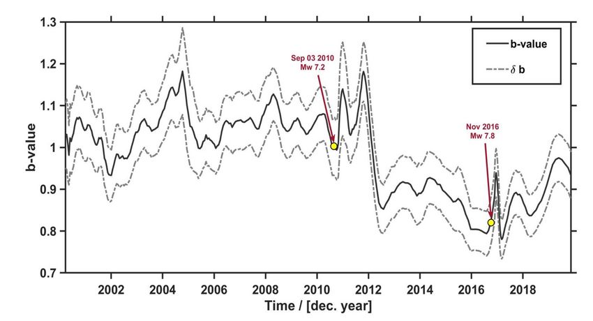
small earthquakes. According to Urbancic (1992), the size distribution of earthquakes quantified by b-
value is possibly a proxy to differentiate stress conditions and could consequently act as a crude stress-
meter wherever seismicity is observed. Thus, the b-value is often interpreted as an indicator of applied
shear stress and material heterogeneity. Several studies (Wyss et al., 2000; Schorlemmer et al., 2004;
Nuannin et al., 2005; Wyss and Stefansson, 2006; Ghosh et al., 2008; Nuannin et al.,2012) have proven
that spatial and temporal b-value anomalies precede the prevalence of large earthquakes. For the reason
that Kaikoura earthquake of Mw 7.8 was a major event in the region with a complex tectonic mechanism,
the b-value anomalies concomitant with this event is of great interest in terms of earthquake
investigation. These anomalies, if any present, will shed light on the stress distribution of the region.
Numerous studies (Scholtz, 1968; Wyss, 1973; Wu et al,. 2008b; Nanjo et al., 2012) suggest a decrease in
b-value with durations of months and years interpreted as boom in stress prior to the occurrence of a
main event. This could mean that low b-values can be expected near the hypocenters of future
earthquakes. In this study, we attempt to probe the variation of Gutenberg-Richter b-value, both spatial
and temporal, and explore the disparity of the pre and post seismic crustal stress conditions associated
to 2016 Mw 7.8 Kaikoura earthquake, northeastern south Island of New Zealand (Fig. 1).

2. Tectonic Settings Of Central New Zealand
The country of New Zealand straddles the boundary between the active obliquely convergent Pacific-
Australian plates which converge at rates of 39–48 mm/yr (Beavan et al., 2002). The opposite-dipping
Hikurangi subduction systems linked by the Alpine Fault transform through MFS provides a sufficiently
large seismicity across New Zealand. In a comparatively short, documented period, the numerous active
faults associated with these plate boundaries have produced frequent large earthquakes in New Zealand.
The relative plate motion changes from slightly oblique subduction of the Pacific Plate beneath the
Australian Plate at a rate close to 50 mm/yr in the northeast of north Island to transpression and very
oblique continental collision at a rate < 40 mm/yr in the south Island (DeMets et al., 2010).

The Mw 7.8, 2016 Kaikoura earthquake occurred within the area of transition between the southern
Hikurangi Subduction Zone and the oblique continental collision along the Alpine Fault (Fig. 1). The MFS
and NCD collectively mark this transition. The MFS includes four major right-lateral strike-slip faults from
north to south, the Wairau, Awatere, Clarence and Hope faults. The faults within this system head
southwards and converge to form the Alpine fault. The Alpine fault, a 650-km-long dextral strike-slip fault
is a main tectonic feature of the south Island. Several dextral faults cut through the upper South Island
and much of the north Island. The focal mechanism solution (U.S. Geological Survey, 2016) indicates
that the preferred fault plane of the strikes northeast roughly parallel to the coastline with a down-dip
toward northwest direction. The event occurred along the multi-segmented faults of around 12 faults in a
combination of different orientations and slip mechanisms. The rupture of the event has propagated
from southwest to northeast along with strike-slip extending over the rupture length of ~170 km from the
epicenter (Duputel & Rivera, 2017; Hamling et al., 2017; Nicol et al., 2018; Xu et al., 2018). The aftershock
zone comprises of the epicenter near the Humps Fault zone and progressing northeastward through the

                                                   Page 3/19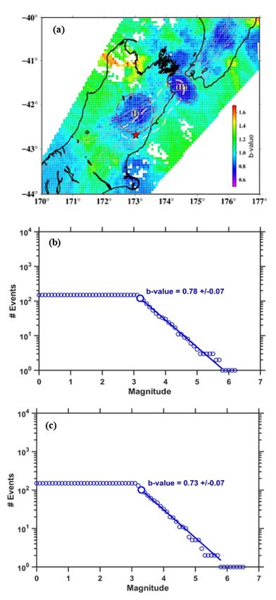
Hundalee Fault, the Hope fault, the Jordan thrust, the Papatea Fault and the Kekerengu fault before
stopping at the Cook Strait. The region has seen experienced several large M > 7 earthquakes in the past
like the 1848 Marlborough earthquake, 1855 Wairarapa earthquake, 1888 Amuri earthquake 1929 Arthurs
pass earthquake etc. Several earthquakes of magnitudes between 6 and 7 has been recorded in the
region too.

3. Data And B-value Mapping
The earthquake size distribution in the Earth’s crust commonly follows the Gutenberg-Richter power law
(Gutenberg & Richter, 1944). The Gutenberg–Richter law gives a fundamental statistical description of
seismicity as: log10N = a – bM, where a and b are constants, M is the magnitude, and N is the number of
earthquakes that occur in a specific time window with magnitude ≥ M. According to this law, a lower b-
value means that larger earthquakes will dominate over smaller earthquakes and a higher b-value means
that there is dominance of small earthquakes over large earthquakes.

The completeness of the earthquake catalog used is important for accurate b-value estimations
(Nuannin, et al., 2012). This is achieved by the estimation of magnitude of completeness (Mc) which is
the smallest magnitude at which the catalog is thought to have included all seismic events. An
underestimate of Mc can result in too low b-value while a larger Mc value increases the uncertainty in b-
value estimation. Among different techniques for Mc calculation, Mc for this catalog is calculated using
maximum curvature method (Wiemer&Wyss,2000). To remove the dependent events like foreshocks and
aftershocks from the catalog, declustering is done. The Reasenberg(1985) algorithm is used for this
purpose.

The b-value is determined by maximum-likelihood method (Aki,1965). To map the spatial variation of b,
earthquake epicenters are projected onto a plane. The b-value is estimated at every node of a plane grid,
using the N (N = constant) nearest earthquakes located within a distance, R, from the node. In this
method, we can ensure a constant sample size for each calculation. The variation of b-value is identified
by creating dense spatial grids and sampling overlapping circular volumes in space and plotting them on
a map. The grid spacing is chosen accordingly so that there is significant overlapping of volumes and
provide a natural smoothening of results.

Temporal b-value variations are calculated by maximum curvature method using sliding time windows
containing a constant number of events. Windows with constant number of events is better than that of
constant time width so that a change in sample size does not affect the calculations.

New Zealand’s GNS Science has been monitoring seismic networks all over the region and it provides
earthquake data. The earthquake catalog for this study was taken from GeoNet service of GNS Science
for the time-period 1st January 2000 to 1st July 2020. It consisted of 17231 events with magnitudes
between 3 and 7.8 and depth from 0 to 350 km. Catalog consisted of magnitude types Mw, mb and ML. To
make the catalog homogeneous, mb and ML were converted to Mw.

                                                 Page 4/19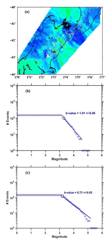
The catalog has been divided into two sub- catalogs: first one with events before the 2016 event
beginning from January 1, 2000 (Fig. 2a) and second one with earthquakes after the event until July 1,
2020 (Fig. 2b). The number of events used for the pre seismic stress field analysis is much higher than
the data used for the post seismic analysis. However the number of events we have considered for both
the cases are sufficient for the estimation of b-value calculations (Zhao and Wu, 2008; Meng et al., 2018).
The calculations are carried out using ZMAP software package (Wiemer, 2001).

4. Results And Discussion
It is globally established that b-value from the Gutenberg-Richter relationship decreases with increasing
differential stress level (Scholz, 1968; Scholz, 2015). To understand the stress configuration of the study
area, we estimate the b-value variations before and after the 2016 Kaikoura earthquake. We apply the
maximum-likelihood method, which has been proved to be a robust and unbiased method in most cases
(Wiemer 2001), to compute the b-value to events in the study area. The selected earthquake catalog is
closely examined to analyze the seismicity of the study area. We used magnitude values from 3 to 8 to
obtain the seismicity map of the entire data catalogue for the study area. Histograms of depth and
magnitude are plotted for the entire catalog (Fig. 3a & 3b). The depth of the events considered vary from
0 to 350 km. It may be noted that maximum number earthquakes are located below 20 km depth.
However, the number of earthquake events maximum up to a depth level of ~ 250 km indicates the
deeper level of subduction zone seismic activities in the plate boundary of the study region. The
histogram of magnitude distribution earthquake as a function of time shows that majority of the
earthquake magnitudes are ranging between Mw 3–4 with large magnitudes are fewer in number.

The cumulative rate of events plotted with time in Fig. 4. The cumulative number shows earthquake
events as function of time. It is noticed that the rate of earthquakes was not constant through time. The
earthquakes with highest magnitudes are mostly occurred in the year 2010 (Mw 7.2) and 2016 (Mw 7.8)
where sharp increases in the pattern of cumulative rates are present. The cumulative frequency of
earthquakes as a function of magnitude is shown in Fig. 5. The straight line represents the maximum
likelihood estimate of a and b values based on the events above magnitude of completeness Mc is
determined. The frequency-magnitude distribution (FMD) for the complete catalog showed magnitude of
completeness Mc as 3.1, b-value as 0.87 and a-value as 6.837. All the events with magnitude less than Mc
were removed from the catalog. After removing events below Mc and declustering, the resulting catalog
consisted of 8239 events. This final catalog is used throughout the seismicity analysis in this study.

4.1. Spatial variation of b-value
To examine the spatial distribution of the pre and post seismic b-value, the study area is divided into a
dense spatial grid of 0.050 x 0.050. b-value is calculated for circular epicentral areas centered at grid
nodes where the radii of circular regions vary along the grid to cover a fixed number of events. In this
case, a circular region containing a minimum of 150 nearby events are required to calculate b-value in

                                                  Page 5/19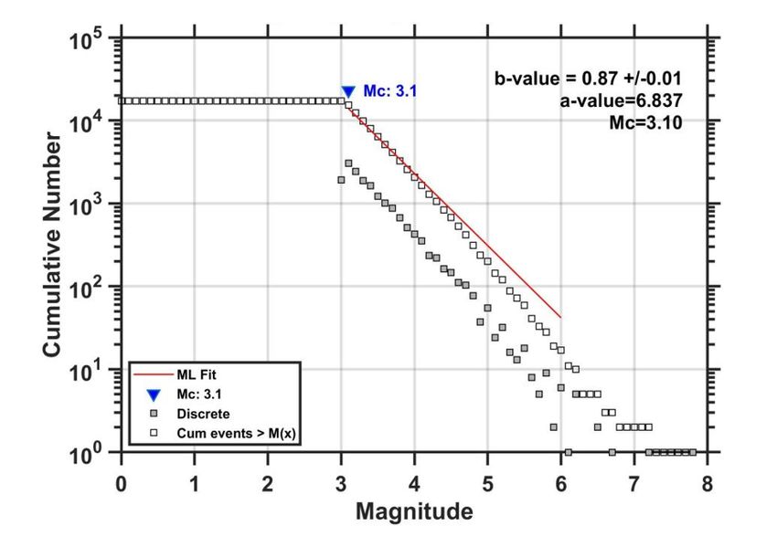
each node. The b-values are calculated by using the Maximum Likelihood method (Aki, 1965). The
calculated pre and post seismic b-values are color coded and plotted as maps in Figs. 6a and 7a.

The b-value map in Fig. 6a shows the pre seismic variation of b-values for a period from the year 2000 to
the day before Mw 7.8 Kaikoura earthquake main-shock. The sub-catalog used for this b-value estimation
consisted of 6809 events (Fig. 2a). The event epicenter and rupture zone associated to the Kaikoura event
are shown in the map. It is evident that two b-value zones are clustered southwest (Zone-I) and northern
(Zone-II) portions of the Kaikoura earthquake rupture zone, suggesting the high stress buildup prior to the
main-shock closer to epicenter and northern end of the rupture respectively. The b-value estimated using
FMD on the nodes placed over this southwest and northern stress fields are 0.78 ± 0.07 and 0.73 ± 0.07
respectively (Figs. 6b and 6c). Figure 7a shows the estimated b-value map for the post seismic period of
the Kaikoura event (i.e from 15th of November 2016 to July 2020). Although the number of events after
the 2016 event is comparatively lower (1427 events) than that of the pre seismic data, they are sufficient
to compute the b-values (Zhao and Wu, 2008; Meng et al., 2018). During the post seismic period, the b-
value of the epicentral node is found to have increased to 1.01 ± 0.08 (Fig. 7b). However, in the northern
part of the rupture zone where the second patch of high stress field demarcated during the pre-seismic
period, the b-value remain same as 0.73 ± 0.05 (Fig. 7c) during the post seismic period as well.

It is established that, before an earthquake low b-value correlates with high stress in the unruptured area.
Vice versa, after an earthquake b-value increases owing to stress releasing in the rupture zone
(Schorlemmer and Wiemer, 2005). Our epicentral mapping of relatively low b-value prior and increase of
b-value later to the Kaikoura earthquake is in good agreement with the studies reported by Wyss et al.
(2000); Wyss and Stefansson (2006); Nanjo et al. (2012); Sreejith et al., 2018, who demonstrated that
triggering range of the large quakes may be mapped by low b-values. However, many studies have
demonstrated that low b-values are indicative of forthcoming large earthquakes (Wiemer and Wyss, 1997;
Schorlemmer and Wiemer, 2005; Sreejith et al., 2018).

Figure 6a shows the southwest cluster of high stress field (Zone–I) near the epicentral area located over
the Marlborough fault systems in the northeastern part of the south Island (Fig. 1). It may be noted that,
the triggering of Kaikoura earthquake was very closely associated to one of the extremely complex
mechanism ever recorded, which involved ~ 12 separate fault segments extending over ~ 170 km from
the epicenter in north Canterbury domain to Cook Strait (Kaiser et al., 2017). Investigation using the field
observations in conjunction with interferometric synthetic aperture radar, Global Positioning System, and
seismology data reveal the propagation of the rupture from south Hope fault to north Cook Strait region
(Hamiling et al., 2017). It is also reported that the northward propagation of the rupture along these
numerous faults was the result of static stress stored over a period of time during the interseismic period
due to the right-lateral oblique-slip movements in north Canterbury and right-lateral strike-slip motions in
the Marlborough fault system (Jiang et al., 2018). Thus our pre seismic analysis result supports the
findings, which state that large areas of high stress accumulation were formed when all of these oblique
and right lateral strike slip motions on crustal faults were employed to stress the shallow fault interface
source of north Canterbury domain and Marlborough fault systems.
                                                  Page 6/19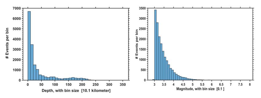
However after the earthquake the high pre seismic stress field demarcated is has changed to
comparatively a stress free zone due to the stress release during the co seismic rupturing (Fig. 7a). The
co seismic deformation taken place not only along the shallow crustal faults of the Marlborough fault
systems but also to some extent at the Hikurangi subduction interface, which slowly released the energy
(Jiang et al., 2018). However in both cases, there is a clear existence of high stress field (low b-value) in
the Zone-II located over the north end of the rupture zone at Cook Strait closer to the Wellington area in
southwestern part of the north Island. Jiang et al. (2018) reported from GPS observations that no
effective co seismic and post seismic deformations associated with the Kaikoura event encouraged to
release the accumulated stress in Cook Strait and neighboring Wellington area.

The Cook Strait has been considered a potential region for frequent earthquakes by many researchers
(Wallace et al., 2009; Pondard and Barnes 2010). The tectonics of Cook Strait is mainly controlled by the
transition of subduction in the north island to transpression in the northern South Island through
numerous fault lines. Using GPS, Seismological and Geological data Wallace et al. (2009) reported that,
Cook Strait province is having a potential to trigger an earthquake of ~ Mw 8.5. However, during 2013 Mw
6.6 Cook Strait earthquake and allied events sequence, released on only a part of the reported energy
(Pondard and Barnes 2010). Thus a good correlation of strain rate obtained from the GPS observations
(Jiang et al., 20018) and b-value estimated in the present study clearly indicate an ongoing strain buildup
in the Cook Strait and Wellington regions which may trigger a larger earthquake in future.

4.2. Temporal variation of b-value
Several laboratory rock-fracture experiments (Mogi, 1963; Scholz, 1968; Lei, 2003) indicate a systematic
decrease in b-value approaching the time of entire fracture. Investigation by Henderson et al., (1994) in
the southern Californian region also supports this result, that seismicity preceding large main-shocks can
be associated with low b-values. In the light of these results, we also evaluated the temporal variation of
b-values (Fig. 8) in terms of earthquakes FMD in the study region for the past two decades. The b-values
are calculated in successive time windows containing a constant number of events N. The window is
moved in time by 10% increments of time. A moving window of 250 events with a minimum of 50 events
and an overlap of 10% increments of events is used.

The events considered span for the period January 1, 2000 to July 1, 2020 with M > 3. In this period, two
large earthquakes of magnitude M > 7 has occurred in the region. The b-value in the region varies between
0.7 and 1.2 and this range of values are consistent with the b-values obtained in the spatial analysis. We
can see that before each M > 7 event that occurred in the region, the trend of the b-value decreases. Also
the b-value of the region has remained below 1 for most of the major events in the past two decade
suggesting that the region was under considerable stress building during this period. The lowest b-value
(~ 0.71) is observed just before the 2016 Kaikoura earthquake for the entire region. It is known that before
any major earthquakes, the b-value is considerably below 1. In a usual case, it is observed that the b-value
decreases before a main event and then slightly increases after the event (Schorlemmer and Wiemer
2005). It may be noted that, before the Mw 7.8 Kaikoura event, the largest earthquake was Mw 7.2

                                                   Page 7/19
Canterbury earthquake on 3rd September 2010 (Atzori et al., 2012). Figure 8 portrays that, there was a
slight decrease in b-value below one prior to Canterbury main event (Shcherbakov et al., 2012).
Conversely there was a slight increase in b-value after the 2010 event. However, the average value
remains well below 1 and keeps decreasing to mark the lowest b-value (~ 0.71) just before the major
event of Mw7.8 in 2016. In the same mode, there is also a slight increase in the b-value after the Kaikoura
earthquake. However, it is similarly noticeable that the b-value in the region has not risen above 1 after the
Kaikoura event. Thus, this could be a sign of an impending earthquake towards Cook Strait province. This
is consistent with the low b-value determined in the spatial variation map of the region after the Kaikoura
main-shock (Fig. 7). Thus the change in b-value can be used as a stress-meter for an impending
earthquake in future (Zang et al., 1998; Lei, 2003; Schorlemmer and Wiemer, 2005).
5. Conclusions
The slope of the relation among frequency-magnitude distributions (FMD) is theoretically 1, however it
often indicates deviations from 1 relies upon the heterogeneity of the area. In order to compare the pre
and post seismic stress variations of in the context of the complex rupturing and mechanism of 2016 Mw
7.8 Kaikoura earthquake, spatial and temporal variations of the earthquake b-values earlier and later to
the main-shock are analyzed. The FMD for the entire catalog confirmed magnitude of completeness Mc
as 3.1, b-value as 0.87 and a-value as 6.837. The analysis of the pre seismic data envisioned a low b-
value with the vicinity of the epicenter at the outer edge of the cluster advocate a high stress
accumulation prior to the main event. Conversely, the presence of a subsequent low b-value cluster
identified to the north of Kaikoura rupture zone during pre and post seismic periods portrays an
unreleased strain energy after the Kaikoura quake rupturing. The assessment of the temporal variations
of b-values for almost two decades strengthened the consistency of the spatial b-value patterns before
and after the major earthquake events in the study region propose that the change in b-value can be used
as a stress-meter for an impending earthquake in destiny.
Declarations
Declaration of competing interest
The authors declare that they have no known competing financial interests or personal relationships that
could have appeared to influence the work reported in this paper.
Acknowledgements
The authors express deep gratitude to Department of Marine Geology and Geophysics, School of Marine
Sciences, Cochin University of Science and Technology (CUSAT) for providing necessary facilities to carry
Page 8/19out this work. T.S. duly acknowledges CUSAT for providing the research fellowship. Most of the figures
are prepared by Generic Mapping Tool (GMT) software.
References
Aki K (1965) Maximum likelihood estimate of b in the formula logN = a-bM and its confidence. Bulletin
Earthquake Research Institute University Tokyo 43:237–239
Atzori S, Tolomei C, Antonioli A, Merryman Boncori JP, Bannister S, Trasatti E, Pasquali P, Salvi S
(2012) The 2010–2011 Canterbury, New Zealand, seismic sequence: Multiple source analysis from InSAR
data and modeling, J. Geophys. Res., 117, B08305, doi:10.1029/2012JB009178, 2012
Bayrak E, Yılmaz Ş, Bayrak Y (2017) Temporal and spatial variations of Gutenberg-Richter parameter
and fractal dimension in Western Anatolia. Turkey J Asian Earth Sci 138:1–11.
https://doi.org/10.1016/j.jseaes.2017.01.031
Beavan J, Tregoning P, Bevis M, Kato T, Meertens C (2002) Motion and rigidity of the Pacific Plate and
implications for plate boundary deformation. J Geophys Res 107(B10):2261.
https://doi.org/10.1029/2001JB000282
Cao A, Gao SS (2002) Temporal variation of seismic b -values beneath northeastern Japan island
arc.Geophys. Res Lett 29, 48-1-48–3. https://doi.org/10.1029/2001gl013775
Chan CH, Wu YM, Tseng TL, Lin TL, Chen CC (2012) Spatial and temporal evolution of b-values before
large earthquakes in Taiwan, 532–535. Tectonophysics, pp 215–222.
https://doi.org/10.1016/j.tecto.2012.02.004
Chen J, Zhu S (2020) Spatial and temporal b-value precursors preceding the 2008 Wenchuan, China,
earthquake (Mw = 7.9): implications for earthquake prediction. Geomatics Nat Hazards Risk 11:1196–
1211. https://doi.org/10.1080/19475705.2020.1784297
DeMets C, Gordon RG, Argus D (2010) Geologically current plate motions. Geophys J Int 181:1–80.
https://doi:10.1111/j.1365-246X.2009.04491
Duputel Z, Rivera L (2017) Long-period analysis of the 2016 Kaikōura earthquake. Phys Earth Planet In
265:62–66
Ghosh A, Newman AV, Thomas AM, Farmer GT (2008) Interface locking along the subduction
megathrust from b-value mapping near Nicoya Peninsula, Costa Rica. Geophy Res Lett 35:L01301.
https://doi:10.1029/2007GL031617
Gutenberg B, Richter CF (1942) Earthquake magnitude, intensity, energy and acceleration. Bull Seismol
Soc Am 32:163–191
Gutenberg B, Richter C (1954) Seismicity of the Earth and Associated Phenomena, 2nded. Princeton
Univ. Press, Princeton, N.J. (310 pp.)
Hamling IJ, Hreinsdóttir S, Clark K, Elliott J, Liang C, Fielding E et al (2017) Complex multifault rupture
during the 2016 Mw 7.8 Kaikōura earthquake, New Zealand. Science 356(6334):eaam7194.
https://doi.org/10.1126/science.aam7194
Page 9/19Henderson J, Main IG, Pearce RG, Takeya M (1994) Seismicity in north-eastern Brazil —fractal
clustering and the evolution of the b-value. Geophys J Int 116:217–226
Ishimoto M, Iida K (1939) Observations of Earthquakes Registered with the Micro Seismograph
Constructed Recently. Bull of the Earthquake Research Institute 17:443–478
Jiang Z, Yuan L, Huang D, Zhang L, Hassan A (2018) Spatial-temporal evolution of slow slip
movements triggered by the 2016 Mw 7. 8 Kaikoura earthquake, New Zealand Tectonophysics 744, 72–
81. https://doi.org/10.1016/j.tecto.2018.06.012
Kaiser A, Balfour N, Fry B, Holden C, Litchfield N, Gerstenberger M et al (2017) The 2016 Kaikoura, New
Zealand, Earthquake: Preliminary Seismological Report. Seismol Res Lett 88(3):727–739.
https://doi.org/10.1785/0220170018
Lanza F, Chamberlain CJ, Jacobs K, Warren-Smith E, Godfrey HJ, Kortink M, Thurber CH, Savage MK,
Townend J, Roecker S, Eberhart-Phillips D (2019) Crustal Fault Connectivity of the Mw 7.8 2016 Kaikōura
Earthquake Constrained by Aftershock Relocations. Geophys Res Lett 46:6487–6496.
https://doi.org/10.1029/2019GL082780
Lay T, Wallace T (1995) Modern Global Seimology
Lei X (2003) How do asperities fracture? An experimental study of unbroken asperities. Earth Planet
Sci Lett 213:347–359. https://doi:10.1016/S0012-821X(03)00328-5
Mogi K (1963) The fracture of a semi-infinite body caused by an inner stress origin and its relation to
the earthquake phenomena (Second Paper), Bull. Earthquake Res Inst Univ Tokyo 41:595–614
Montuori C, Falcone G, Murru M, Thurber C, Reyners M, Eberhart-Phillips D (2010) Crustal
heterogeneity highlighted by spatial b-value map in the Wellington region of New Zealand. Geophys J Int
183:451–460. https://doi.org/10.1111/j.1365-246X.2010.04750.x
Meng X, Yang H, Peng Z (2018) Foreshocks, b valuemap, and aftershock triggering for the 2011 Mw
5.7 Virginia earthquake. Journal of Geophysical Research: Solid Earth 123:5082–5098.
https://doi.org/10.1029/2017JB015136
Nanjo KZ, Hirata N, Obara K, Kasahara K (2012) Decade-scale decrease in b value prior to the M9-class
2011 Tohoku and 2004 Sumatra quakes. Geophys Res Lett 39:3–6.
https://doi.org/10.1029/2012GL052997
Nanjo KZ, Yoshida A (2018) A b map implying the first eastern rupture of the Nankai Trough
earthquakes. Nat Commun 9(1):3–6. https://doi.org/10.1038/s41467-018-03514-3
Nicol A, Khajavi N, Pettinga JR, Fenton C, Stahl T, Bannister S, Pedley K, Hyland-Brook N, Bushell T,
Hamling I, Ristau J, Noble D, McColl ST (2018) Preliminary geometry, displacement, and kinematics of
fault ruptures in the epicentral region of the 2016 Mw 7.8 Kaikōura, New Zealand, earthquake. Bull
Seismol Soc Am 108(3B):1521–1539. https://doi.org/10.1785/0120170329
Nuannin P, Kulhanek O, Persson L (2005) Spatial and temporal b value anomalies preceding the
devastating off coast of NW Sumatra earthquake of December 26, 2004. Geophys Res Lett 32(11):1–4.
https://doi.org/10.1029/2005GL022679
Page 10/19Nuannin P, Kulhánek O, Persson L (2012) Variations of b-values preceding large earthquakes in the
Andaman-Sumatra subduction zone. J Asian Earth Sci 61:237–242.
https://doi.org/10.1016/j.jseaes.2012.10.013
Pondard N, Barnes PM (2010) Structure and paleo-earthquake records of active submarine faults,
Cook Strait, New Zealand: Implications for fault interactions, stress loading, and seismic hazard. J
Geophys Res:Solid Earth 115(12):1–31. https://doi.org/10.1029/2010JB007781
Reasenberg PA (1985) Second-order moment of central California seismicity, 1969–1982. J Geophys
Res 90:5479–5495
Scholz CH (1968) The frequency-magnitude relation of micro fracturing in rock and its relation to
earthquakes. Bull Seismol Soc Am 58:399–415
Scholz CH (2015) On the stress dependence of the earthquake b value. Geophys Res Lett 42:1399–
1402. https://doi.org/10.1002/2014GL062863
Schorlemmer D, Wiemer S (2005) Microseismicity data forecast rupture area. Nature 434:1086
Schorlemmer D, Wiemer S, Wyss M (2005) Variations in earthquake-size distribution across different
stress regimes. Nature 437:539–542. https://doi.org/10.1038/nature04094
Shcherbakov R, Nguyen M, Quigley M (2012) Statistical analysis of the 2010 MW 7.1 Darfield
Earthquake aftershock sequence. NZ J Geol Geophys 55(3):305–311
Shi X, Wang Y, Liu-Zeng J, Weldon R, Wei S, Wang T, Sieh K (2017) How complex is the 2016 Mw 7.8
Kaikoura earthquake, South Island. New Zealand? Sci Bull 62(5):309–311.
https://doi.org/10.1016/j.scib.2017.01.033
Sreejith KM, Sunil PS, Agrawal R, Saji AP, Rajawat AS, Ramesh DS (2018) Audit of stored strain energy
and extent of future earthquake rupture in central Himalaya. Sci Rep 8:1–9.
https://doi.org/10.1038/s41598-018-35025-y
Stirling M, McVerry G, Gerstenberger M, Litchfield N, Van Dissen R, Berryman K, Barnes P, Wallace L,
Villamor P, Langridge R, Lamarche G, Nodder S, Reyners M, Bradley B, Rhoades D, Smith W, Nicol A,
Pettinga J, Clark K, Jacobs K (2012) National seismic hazard model for New Zealand: 2010 update. Bull
Seismol Soc Am 102:1514–1542. https://doi.org/10.1785/0120110170
Urbancic TI, Feignier B, Young RP (1992) Influence of source region properties on scaling relations for
M < 0 events. PAGEOPH 139:721–739. https://doi.org/10.1007/BF00879960
Wallace LM et al (2009) Characterizing the seismogenic zone of a major plate boundary subduction
thrust: Hikurangi Margin, New Zealand, Geochem Geophys Geosyst,10,Q10006,
https://doi:10.1029/2009GC002610
Wallace LM, Barnes P, Beavan J, Van Dissen R, Litchfield N, Mountjoy J, Langridge R, Lamarche G,
Pondard N (2012) The kinematics of a transition from subduction to strike-slip: An example from the
central New Zealand plate boundary. J Geophys Res: Solid Earth, 117(2).
https://doi.org/10.1029/2011JB008640
Wiemer S (2001) A software package to analyze seismicity: ZMAP. Seismol Res Lett 72:373–382
Page 11/19Wyss M (2001) Locked and creeping patches along the Hayward Fault, California. Geophys Res Lett
28:3537–3540. https://doi.org/https://doi.org/10.1029/2001GL013499
Wyss M, Stefansson R (2006) Nucleation Points of Recent Mainshocks in Southern Iceland, Mapped
by b-Values. Bull Seismol Soc Am 96:599–608. https://doi.org/10.1785/0120040056
Xu W, Feng G, Meng L, Zhang A, Ampuero JP, Burgmann R, &Fang L (2018) Transpressional rupture
cascade of the 2016 Mw 7.8 Kaikoura earthquake, New Zealand. J Geophys Res: Solid Earth 123:2396–
2409. https://doi.org/10.1002/2017JB015168
Yarce J, Sheehan AF, Nakai JS, Schwartz SY, Mochizuki K, Savage MK, Wallace LM, Henrys SA, Webb
SC, Ito Y, Abercrombie RE, Fry B, Shaddox H, Todd EK (2019) Seismicity at the Northern Hikurangi Margin,
New Zealand, and Investigation of the Potential Spatial and Temporal Relationships With a Shallow Slow
Slip Event. J Geophys Res: Solid Earth 124(5):4751–4766. https://doi.org/10.1029/2018JB017211
Zang A, Wagner FC, Stanchits S, Dresen G, Andresen R, Haidekker M (1998) Source analysis of
acoustic emissions in Aue granite cores under symmetric compressive loads. Geophys J Int 135:1113–
1130
Figures
Page 12/19Figure 1
Map represents tectonic setup of the study region with the epicenter location (red star) of 14 November
2016 (Mw 7.8) Kaikoura, New Zealand earthquake. A few days aftershocks above Mw 4.0 of the event as
a function of depth are presented with colored circles. The size of the circle represents the different
magnitudes. The blue colour beach ball indicates the oblique thrust faulting focal mechanism solution
(U.S. Geological Survey 2016). Continuous black lines indicate the active fault systems and subduction
zones of the region. The white arrow represents the co-seismic rupture propagation direction towards
northeast from the epicenter.
Page 13/19Figure 2
(a) Pre seismicity and (b) post seismicity of the region used the FMD analysis before and after the Mw
7.8 Kaikoura earthquake. The colour indicates the focal depth of the events.
Figure 3
Histograms showing the earthquake events distribution (a) as a function of Depth and (b) as a function
of Magnitude used in the present study.
Page 14/19Figure 4
Cumulative rate of seismic events in the study as a function of time. Yellow stars indicate larger
earthquakes Mw 7.2 and Mw 7.8 occurred during 2010 and 2016, respectively.
Page 15/19Figure 5
Frequency-Magnitude distributions for the entire catalog shown by the cumulative distribution. The
determined Cutoff magnitude Mc = 3.10. Red line shows the fitting of Gutenberg-Richter’s law.
Page 16/19Figure 6
(a) Spatial distribution map of b-value variation from 1 January 2000 to the day before the Mw 7.8
Kaikoura earthquake. The star indicates the epicenter location and white colour dashed polygon indicates
the rupture area of the Kaikoura main-shock. The red colour dashed open circles indicates the pre seismic
high stress field areas (low b-value zones) prior to the main-shock. (b) Pre seismic FMD at Zone-I node
and (c) Pre seismic FMD at the Zone-II node.
Page 17/19Figure 7
(a). Spatial distribution map of b-value variation after the Kaikoura earthquake to 31 July 2020. The star
indicates the epicenter location and white colour dashed polygon indicates the rupture area of the
Kaikoura main-shock. The red colour dashed open circle (I) indicates the post seismic stress released
area (high b-value) and open circle (II) indicates the post seismic high stress filed area (low b-value) after
the main-shock. (b) Post seismic FMD at Zone –I node and (c) Post seismic FMD at Zone II node.
Page 18/19Figure 8
Temporal variation plot of b-value with time from 1st January 2000 to 31st July 2020. Yellow stars
indicate two large earthquake events during the period. The gray dash lines indicate the standard
deviation of the estimated b-value.
Page 19/19You can also read