A Computational Framework for Quantifying and Analyzing System Flexibility
←
→
Page content transcription
If your browser does not render page correctly, please read the page content below
A Computational Framework for Quantifying and
                                                                             Analyzing System Flexibility
                                                                     Joshua L. Pulsipher, Daniel Rios, and Victor M. Zavala*
                                                                            Department of Chemical and Biological Engineering
arXiv:2106.12706v1 [math.OC] 24 Jun 2021

                                                                  University of Wisconsin, 1415 Engineering Dr, Madison, WI 53706, USA

                                                                                                  Abstract

                                                      We present a computational framework for analyzing and quantifying system flexibility. Our
                                                  framework incorporates new features that include: general uncertainty characterizations that are
                                                  constructed using composition of sets, procedures for computing well-centered nominal points,
                                                  and a procedure for identifying and ranking flexibility-limiting constraints and critical parameter
                                                  values. These capabilities allow us to analyze the flexibility of complex systems such as distribu-
                                                  tion networks.

                                           Keywords: flexibility; uncertainty; complex systems

                                           1    Introduction and Basic Terminology
                                           This report details proposed extensions in characterizing the flexibility of physical systems subjected
                                           to uncertainties. Such uncertainty may stem from a wide variety of sources including the system’s
                                           environment (e.g., ambient temperature, product demand) and the system itself (e.g., kinetic con-
                                           stants, battery life). Flexibility denotes the capability of a system to maintain feasible operation over
                                           a range of uncertain/random conditions [27]. This becomes prevalent in many applications such
                                           as chemical processes [19, 25], power systems [17, 28], and autonomous vehicles [14, 29] where it is
                                           critical that sufficient flexibility is engineered into system design to promote profitability and safety.
                                           For instance, chemical plants encounter numerous uncertainties (e.g., feed flowrates, heat transfer
                                           coefficients, equipment fatigue) that can induce costly failures for designs that are not sufficiently
                                           flexible [3]. Accounting for flexibility can also help reduce design costs, since accurate analysis of
                                           a system’s flexibility helps to prevent the over-engineering that has prevailed traditional chemical
                                           process design practices [27].
                                               A number of approaches have been previously proposed to quantify system flexibility and an
                                           extensive review is provided in [10]. The stochastic flexibility index, originally proposed by Straub
                                           and Grossmann, is a flexibility metric for systems that are subjected to uncertain parameters (e.g.,
                                           disturbances, physical parameters) that are modeled as random variables [26]. Pistikopoulos and
                                               * Corresponding   Author: victor.zavala@wisc.edu

                                                                                                     1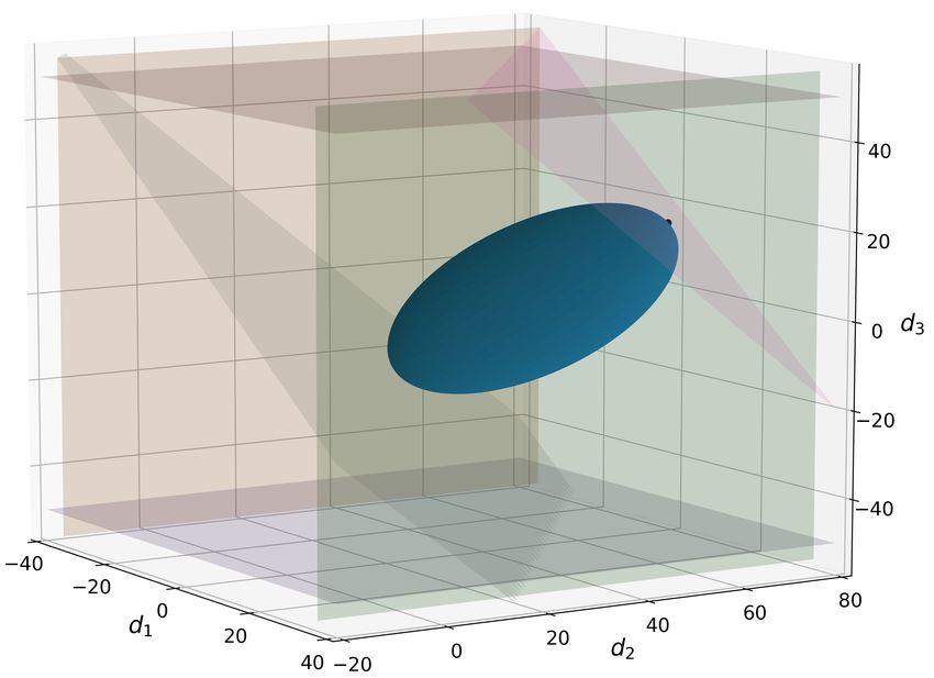
http://zavalab.engr.wisc.edu

Mazzuchi propose a similar metric in [20]. The stochastic flexibility index SF is defined as the prob-
ability of finding recourse to maintain feasible operation (i.e., the probability of satisfying all the
system constraints). This can be computed by integrating the probability density function of the
random parameters over the feasible region:
                                                     Z
                                          SF :=              p(θ)dθ                                  (1.1)
                                                      θ∈Θ

where θ ∈ Rnθ is a realization of the random parameters, Θ := {θ : ψ(θ) ≤ 0} is the feasible set of
the system and p : Rnθ → R is the probability density of the parameters. The function ψ(θ) evaluates
the feasibility of the system for a given realization of θ and is given by:

                                 ψ(θ) := min max fj (z, x, θ)
                                            z,x j∈J
                                                                                                     (1.2)
                                            s.t. hi (z, x, θ) = 0, i ∈ I,

where z ∈ Rnz are the system recourse variables, x ∈ Rnx are the system state variables, fj (z, x, θ), j ∈
J are the system inequality constraint functions and hi (z, x, θ), i ∈ I are the system equality con-
straint functions. The system is deemed feasible at a given realization of θ if ψ(θ) ≤ 0 (this implies
that fj (z, x, θ) ≤ 0 and hi (z, x, θ) = 0 hold for all i ∈ I and j ∈ J). The system is infeasible at
θ if ψ(θ) > 0. The boundary of the feasible region is given by the set ∂Θ := {θ | ψ(θ) = 0}. In
other words, at a given realization θ, the system is at the boundary of the feasible region if ψ(θ) = 0.
Problem (1.1) can also be expressed as:

             SF = P (ψ(θ) ≤ 0) = P ∃ z, x : max fj (z, x, θ) ≤ 0, hi (z, x, θ) = 0, i ∈ I .          (1.3)
                                                j∈J

From this representation, we can see that the SF index is a joint chance constraint [22].
    The SF index can be computed rigorously by evaluating (1.1) via Monte Carlo (MC) sampling.
This is done by assessing the feasibility of each realization. Such an approach converges exponen-
tially with the number of MC samples but typically requires a very large number of samples [24, 23].
Straub and Grossmann presented a quadrature technique to reduce the number of samples required,
but quadrature methods still suffer from scalability issues [26, 7].
    The so-called flexibility index problem, first proposed by Grossmann et. al. [12], provides a more
scalable approach to quantifying flexibility. This approach seeks to identify the largest uncertainty
set T (δ) (where δ ∈ R+ is a parameter that scales T ) for which the system remains feasible. In
other words, we seek to find the largest uncertainty set under which there exists recourse to recover
feasibility. The flexibility index F is defined as:

                                     F := max δ
                                            δ∈R+
                                                                                                     (1.4)
                                              s.t.       max ψ(θ) ≤ 0.
                                                         θ∈T (δ)

This approach is deterministic in nature; consequently, it does not have a direct probabilistic inter-
pretation (as the SF index does). For convenience, ψ(θ) can be reformulated by using an upper

                                                         2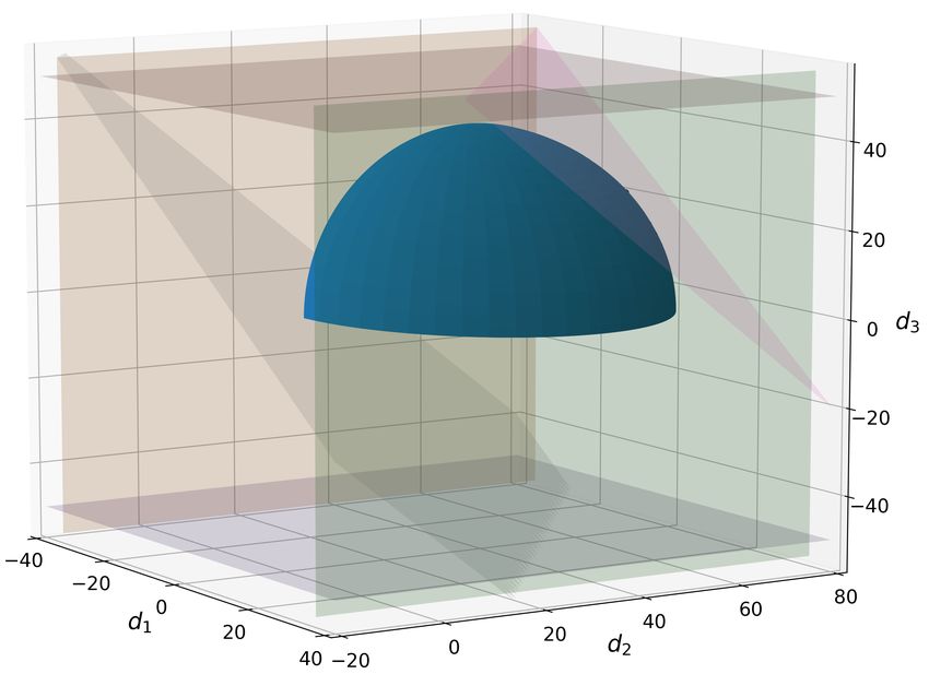
http://zavalab.engr.wisc.edu

bounding variable u ∈ R:

                                 ψ(θ) = min u
                                           z,x,u

                                            s.t. fj (z, x, θ) ≤ u, j ∈ J                             (1.5)

                                                   hi (z, x, θ) = 0, i ∈ I.

Problem (1.4) is a bi-level optimization problem that seeks to find the largest uncertainty set T (δ) that
can be inscribed in the feasible region defined by Θ. Figure 1 illustrates the index F for an inequality
system using a hyperbox uncertainty set which is described further below in Equation (1.8).

         Figure 1: Illustration of flexibility index problem under a hyperbox uncertainty set.

     Swaney and Grossmann [27] proved that Problem (1.4) is equivalent to searching for the min-
imum δ along the boundary ∂Θ, provided that T (δ) is compact and the constraints fj (z, x, θ) and
hi (z, x, θ) are Lipschitz continuous in z, x, and θ. Thus, (1.4) can be expressed as:

                                     F =           min       δ
                                            δ∈R+ , θ∈T (δ)
                                                                                                     (1.6)
                                                         s.t. ψ(θ) = 0.

    Grossmann and Floudas leverage this observation to propose a mixed-integer program (MIP) that
casts the constraint ψ(θ) = 0 in terms of its first-order Karush-Kuhn-Tucker (KKT) conditions [11].
The MIP is given by:

                                                         3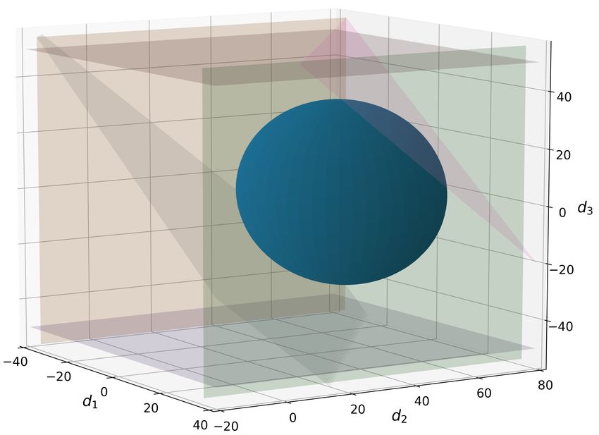
http://zavalab.engr.wisc.edu

             F =            min              δ
                    δ,z,x,θ,λj ,sj ,yj ,µj

                                     s.t. fj (z, x, θ) + sj = 0                            j∈J
                                             hi (z, x, θ) = 0                              i∈I
                                             X
                                                  λj = 1
                                             j∈J
                                             X          ∂fj (z, x, θ) X ∂hi (z, x, θ)                 (1.7)
                                                   λj                + µi             =0
                                                             ∂z              ∂z
                                             j∈J                    i∈I

                                             sj ≤ U (1 − yj )                              j∈J
                                             λj ≤ yj                                       j∈J
                                             θ ∈ T (δ)
                                             λj , sj ≥ 0; yj ∈ {0, 1}                      j ∈ J.

where sj , λj are slack variables and Lagrange multipliers for the inequality constraints fj (z, x, θ), and
yj are binary variables that indicate if the corresponding inequality constraints are active or inactive.
Symbol µi denotes Lagrange multipliers for the equality constraints hi (z, x, θ). The constant U is
a suitable upper bound for the slack variables. Problem (1.7) provides a tractable formulation to
compute the index F that provides a global solution when the convexity conditions presented by
Grossmann and Floudas are satisfied (i.e., Θ is a convex set) [11]. Global solutions for nonlinear
systems that do not satisfy these convexity conditions can still be obtained if a global optimization
algorithm is applied such as the αBB branch-and-bound algorithm employed by Floudas et. al. in [6].
The flexibility index problem also shares some common ground with robust optimization methods,
Zhang et. al. discuss this relationship in detail for linear systems [31].
   Because of the difficulty in parameterizing the uncertainty set in terms of a scalar variable δ, the
majority of studies reported in the literature use a hyperbox representation of the uncertainty set:

                                   Tbox (δ) = {θ : θ̄ − δ∆θ − ≤ θ ≤ θ̄ + δ∆θ + }                      (1.8)

where θ̄ is a nominal point and ∆θ − , ∆θ + are maximum lower and upper deviations, respectively
[10]. In conjunction with Problem (1.7), this set provides a straightforward interpretation of the flex-
ibility index (which we denote as Fbox where the subscript indicates what uncertainty set is used in
combination with Problem (1.7)). Specifically, Fbox ≥ 1 indicates that the design is sufficiently flexi-
ble for the specified deviations. The limitations with the hyperbox set are that it requires upper and
lower bounds to be assigned to each random parameters (which may be arbitrary in applications)
and that it does not capture correlations between random parameters.
    Recently, Pulsipher and Zavala [22] showed that any compact set representation of T (δ) can be
utilized in combination with Problem (1.7). In particular, they showed that an ellipsoidal uncertainty
set is the natural choice for T (δ) when the uncertain parameters are multivariate Gaussian variables
θ ∼ N (θ̄, Vθ ) (where θ̄ is the mean and Vθ is a positive definite covariance matrix). The ellipsoidal
uncertainty set is given by:

                                                                4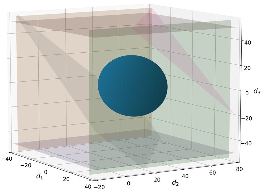
http://zavalab.engr.wisc.edu

                               Tellip (δ) = {θ : (θ − θ̄)T Vθ−1 (θ − θ̄) ≤ δ}.                      (1.9)

   One advantage of using Tellip (δ) in combination with Problem (1.7) is that the associated flexibility
index (denoted by Fellip ) can be used to obtain the confidence level:
                                                           F
                                                    γ( n2θ , ellip
                                                               2 )
                                            α∗ :=           nθ                                     (1.10)
                                                        Γ( 2 )

where γ(·) and Γ(·) are the incomplete and complete gamma functions. Interestingly, this confidence
level provides a lower bound for the stochastic flexibility index SF (i.e., α∗ ≤ SF ) [22]. This thus
provides an avenue to obtain a probabilistic interpretation of the deterministic flexibility index while
avoiding MC sampling and quadrature schemes.
    This paper describes extensions to the aforementioned approaches that help establish a frame-
work for analyzing flexibility of complex systems. These extensions include a generalization of the
uncertainty set representation by using intersecting sets, systematic approaches for obtaining nomi-
nal points, and a methodology for identifying and ranking flexibility-limiting constraints. The paper
is structured as follows: in Section 2 we establish and describe our proposed extensions. Section 3
illustrates the concepts by using small and large distribution networks.

2     Flexibility Analysis Framework
This section describes the components of a flexibility analysis framework. The framework incorpo-
rates extensions to enable distinct characterizations of T (δ), to select θ̄, to compare system designs,
and to identify and rank limiting constraints.

2.1   Uncertainty Set Characterizations

Problem (1.7) can use any compact set T (δ) whose size can be parameterized in terms of a scalar
variable δ. The selection of T (δ) will depend on the application and on the nature of the uncertain
parameters θ. In [22], a number of uncertainty sets are provided that can be used in conjunction
with Problem (1.7). Table 1 summarizes such sets. We note that the ellipsoidal norm set in Table
1 is equivalent to Tellip (δ) as defined in (1.9) provided that A = Vθ−1 . The ellipsoidal norm set can
also be used to approximate polytopes [2]. We also note that Tbox (δ) is equivalent to T∞ (δ) when
∆θ −        +
    i = ∆θ i = 1. Li et.al. provide an analysis of the `1 , `2 , and `∞ -norm uncertainty sets along with
their mathematical properties in the context of robust optimization [16]. The conditional value at risk
(CVaR) norm, originally proposed by Pavlikov and Uryasev in [18], has gained interest in the robust
and stochastic optimization communities because of its ability to approximate `p norms via linear
programming (precisely reproducing the `1 and `∞ norms as extreme cases) [9].
    Li et. al. also analyzed sets that result from intersections (compositions) of `p -norm sets (e.g.,
T2 (δ) ∩ T∞ (δ)) [16]. Inspired by this, we observe that T (δ) can be represented by any combination
of the uncertainty sets in Table 1 or other sets (provided that the resulting combined set is compact).
This provides the ability to incorporate physical knowledge on the uncertain parameters and/or to

                                                      5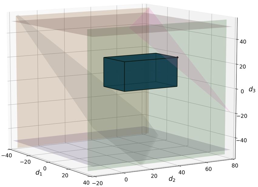
http://zavalab.engr.wisc.edu

                    Table 1: Potential representations for the uncertainty set T (δ).

                         Name                             Uncertainty Set
                   Ellipsoidal Norm             Tellip (δ) = {θ : ||θ − θ̄||2A ≤ δ}
                     Hyperbox Set       Tbox (δ) = {θ : θ̄ − δ∆θ − ≤ θ ≤ θ̄ + δ∆θ + }
                       `∞ Norm                  T∞ (δ) = {θ : ||θ − θ̄||∞ ≤ δ}
                        `1 Norm                  T1 (δ) = {θ : ||θ − θ̄||1 ≤ δ}
                        `2 Norm                  T2 (δ) = {θ : ||θ − θ̄||2 ≤ δ}
                      CVaR norm               TCV aR (δ) = {θ : hhθ − θ̄iiα ≤ δ}

create a wider range of uncertainty set shapes. For instance, the positive (truncated) ellipsoidal set
Tellip+ (δ) := Tellip (δ) ∩ Rn+θ , where Rn+θ := {θ : θ ≥ 0} can be used to represent parameters that are
known to be non-negative (e.g., demands, prices). Similarly, we can define the positive hyperbox
set Tbox+ (δ) := Tbox (δ) ∩ Rn+θ . Compositions of sets can be naturally accommodated in conjunction
with problem (1.7), by imposing the constraints corresponding to each set. For instance, Tellip+ (δ) is
represented by adding the constraints (θ − θ̄)T Vθ−1 (θ − θ̄) ≤ δ and θ ≥ 0 to the MIP formulation.

2.2   Nominal Point Selection Methods

Most uncertainty sets require a nominal point θ̄. The choice of the nominal point θ̄ is critical; for ex-
ample, a nominal point that is close to the boundary of the feasible region will have limited flexibility.
In some applications, specifying θ̄ might be difficult if not enough data is available or if a system is
not routinely operated at any given point (e.g., a power grid). Thus, we introduce methods that can
be employed to find well-centered nominal points. We note that one would be tempted to let θ̄ be
a free variable in Problem (1.7) to find a nominal point but this approach leads to trivial solutions.
This is because the objective is minimized when the nominal point θ̄ is placed on the boundary of θ.
Consequently, this naive approach cannot be used to compute a nominal point.
    We propose an extension of the analytic center (commonly used in interior-point methods) to com-
pute a nominal point. The analytic center θ̄ ac is given by:
                                               X
                            θ̄ ac := argmax         log (sj )
                                     θ,z,x,sj   j∈J
                                                                                                    (2.11)
                                          s.t. fj (z, x, θ) + sj ≤ 0, j ∈ J
                                                hi (z, x, θ) = 0,      i ∈ I.

Here, sj ∈ R are slack variables. This problem pushes the constraints to the interior of the feasible
region. Any bounded solution of the above problem satisfies sj > 0 and thus fj (z, x, θ̄ ac ) < 0 for all
j ∈ J. Consequently, we have that ψ(θ̄ ac ) < 0 and thus θ̄ ac ∈ Θ (the analytic center is feasible). We
also note that the analytic center is the point that maximizes the geometric mean of the constraints
                                                  P
(slack variables). By changing the objective to j∈J sj one finds a center point that maximizes the
arithmetic mean.

                                                      6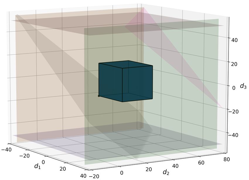
http://zavalab.engr.wisc.edu

      We also propose a center point θ̄ f c (that we call the feasible center) and that we define as:

                                θ̄ f c := argmax s
                                           θ,z,x,s

                                               s.t. fj (z, x, θ) + s ≤ 0, j ∈ J                         (2.12)

                                                     hi (z, x, θ) = 0,       i ∈ I.

Here, s ∈ R is a slack variable. The feasible center is the point that maximizes the worst-case slack
variable (as opposed to the geometric mean used in the analytic center). We also note that θ̄ f c =
argminθ ψ(θ) = argmaxθ −ψ(θ) and that ψ(θ̄ f c ) ≤ 0. Moreover, (2.12) is equivalent to (1.5) when
the parameter θ is set as a free variable.
    The feasible center is an approximation of the center point:

                                            θ̄ d := argmax d(θ, ∂Θ)                                     (2.13)
                                                     θ∈Θ

where d(θ, ∂Θ) = minθ0 ∈∂Θ kθ − θ 0 k. In other words, θ̄ d is the point that maximizes the distance
to the boundary of feasible set. This point is a natural center point but it is difficult to compute
due to the nested max and min operators. We now proceed to show that | − ψ(θ)| provides a lower
bound of d(θ, ∂Θ). Consequently, because the feasible center θ̄ f c maximizes −ψ(θ), we have that
this also implicitly maximizes d(θ, ∂Θ). This property can be established as follows, if the constraints
are Lipschitz continuous (as often assumed in the flexibility analysis literature), we have that ψ(·) is
Lipschitz as well and thus:

                                          |ψ(θ̂) − ψ(θ)| ≤ Lkθ̄ d − θk                                  (2.14)

where θ̂ = argminθ0 ∈∂Θ kθ − θ 0 k for a particular value of θ. Because θ̂ ∈ ∂Θ, we have that ψ(θ̂) = 0
and thus,

                                      |ψ(θ̂) − ψ(θ)| = | − ψ(θ)|
                                                      ≤ Lkθ̂ − θk
                                                      = L min
                                                          0
                                                              kθ 0 − θk
                                                             θ ∈∂Θ

                                                      = L d(θ, ∂Θ).                                     (2.15)

We thus conclude that:
                                                           1
                                            d(θ, ∂Θ) ≥       | − ψ(θ)|.                                 (2.16)
                                                           L
Consequently, maximizing −ψ(θ) implicitly maximizes d(θ, ∂Θ). Moreover, we note that d(θ, ∂Θ) =
−ψ(θ) = 0 if θ ∈ ∂Θ.

2.3     Design Comparison

The flexibility index is a valuable metric that can be used to compare system designs. The utility and
interpretation of the index for a system will depend on the choice of T (δ). For instance, the index

                                                         7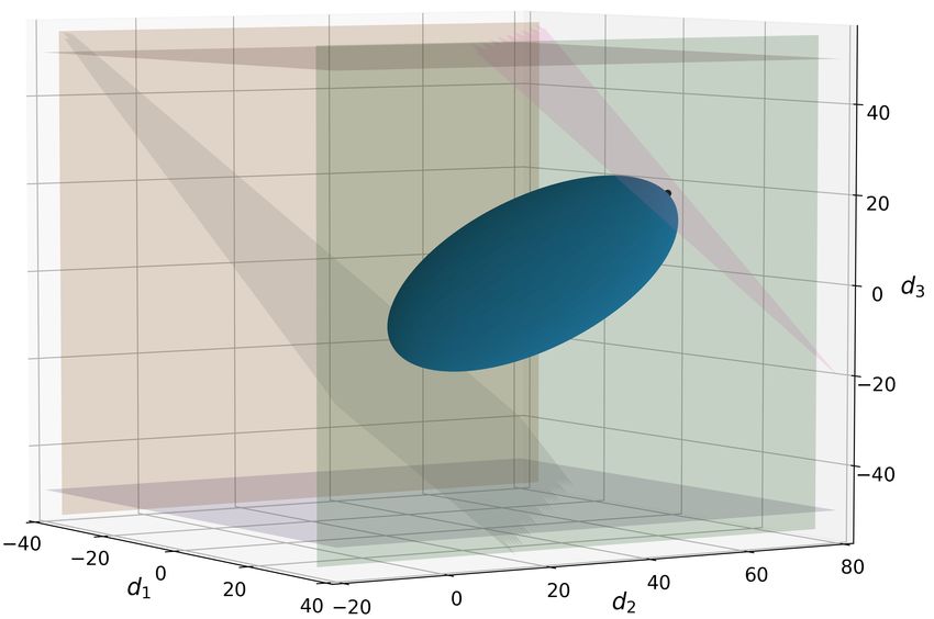
http://zavalab.engr.wisc.edu

can be used to determine the confidence level α∗ if the set Tellip (δ) is used (when θ ∼ N (θ̄, Vθ )). The
index might not have a clear interpretation or utility for some choices of T (δ) but can still be useful
to quantify improvements in flexibility from design modifications (retrofits). We illustrate this feature
by using the following example.
   Consider two system designs that are each subjected to two normal random variables and that
have no recourse variables z as summarized in Table 2.

                        Table 2: System Constraints of Design A and Design B.

                                          Design A                  Design B
                                                             3
                              f1   :   θ 1 + θ 2 − 14 ≤ 0    4 θ1   + θ 2 − 14 ≤ 0
                                                             3
                              f2   :   θ 1 − 2θ 2 − 2 ≤ 0    4 θ1   − 2θ 2 − 2 ≤ 0
                              f3   :        −θ 1 ≤ 0                −θ 1 ≤ 0
                              f4   :        −θ 2 ≤ 0                −θ 2 ≤ 0

The nominal point θ̄ and the covariance matrix Vθ are taken to be:
                                               " #            "  #
                                                4            2 1
                                          θ̄ =          Vθ =       .                                (2.17)
                                                5            1 3

Given that the parameters are multivariate Gaussian, we choose to use Tellip (δ). We also compute
Fbox using Tbox (δ), where ∆θ − and ∆θ + are both taken to be (4.243, 5.196). These bounds correspond
to θ̄ i ± 3σi confidence bounds where σi is the standard deviation of θ i . For comparison, the SF index
is rigorously computed using 100,000 MC samples. Table 3 summarizes the results. Both flexibility
indexes indicate that Design B is more flexible. We also see that the confidence level α∗ also provides
a conservative approximation of SF .

                    Table 3: Comparing the flexibility of Design A and Design B.

                                           Fbox   Fellip    α∗ (%)     SF -MC (%)
                            Design A       0.53      3.57    83.1          96.6
                            Design B       0.66      6.40    95.9          98.9

    Figure 2 depicts the two different systems. It is apparent that Design B has a larger feasible region
Θ and thus has a larger SF index. A key observation is that the choice of T (δ) significantly affects how
it measures system flexibility. For instance, for Design B, the ellipsoidal and hyperbox sets identify
different limiting constraints, and thus exhibit distinct behavior. In particular, index Fbox is limited
by constraint f2 and would not change if constraints f1 , f3 , and/or f4 were varied to increase the
area of Θ, even though the overall system flexibility would be improved. On the other hand, index
Fellip is limited by constraint f1 . This conservative behavior parallels what is observed with the use

                                                        8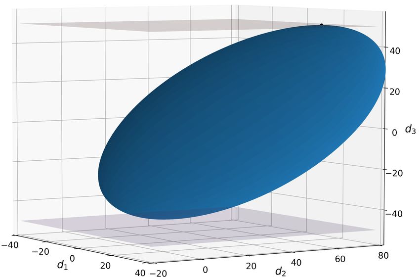
http://zavalab.engr.wisc.edu

of uncertainty sets in robust optimization, where such sets are used to optimize against the worst
case scenario such that the solution is robust in the face of uncertainty, and the conservativeness of a
solution depends on the chosen shape of the uncertainty set [8].

                     (a) Design A                                      (b) Design B

 Figure 2: Elliptical and hyperbox uncertainty sets relative to feasible regions of Designs A and B.

2.4    Limiting Constraint Ranking

An important observation that we make is that the flexibility index problem also implicitly identifies
inequality constraints that limit flexibility. Such information can be valuable in design or operat-
ing procedures. Specifically, at a solution of Problem (1.7), the binary variables yj indicate which
inequality constraints are active and therefore limit flexibility. Problem (1.7) can thus be resolved
by excluding this first set of limiting constraints, so that the next set of limiting constraints can be
identified. This step can be repeated to rank system constraints to a desired extent (as long as the
solution of Problem (1.7) is bounded). This is done by noticing that each set of limiting constraints
will have an associated flexibility index, which indicates how limiting a particular set of constraints
is relative to the other sets. We note that this analysis operates under the assumption that the inequal-
ity constraints can be eliminated/relaxed such that the system still has physical meaning. However,
this assumption is met in many applications since constraints that cannot be removed (e.g., physical
laws) typically correspond to equality constraints.
     This methodology can also be used to identify and rank system components that limit flexibility
in order to guide design improvements or quantify value of specific components, since such iden-
tification is useful to understand and identify system vulnerabilities. Thus, this ranking becomes
useful for complex systems where it is difficult to determine vulnerable components. For example,
this approach can identify which heat-exchangers in a heat-exchanger network could be retrofitted
to most increase the system flexibility, and similarly identify heat-exchangers that would not lead to
increased flexibility when improved. Limiting constraint information can also be used to quantify
the impact of failure of system components (e.g., a production facility).
      This proposed approach shares some common ground with optimal design problems where de-

                                                   9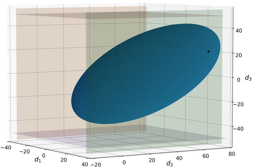
http://zavalab.engr.wisc.edu

sign variables d (added to the system constraints fj (z, x, θ) and hi (z, x, θ)) are selected to minimize
cost and satisfy a specified index F [1, 13, 21]. This provides a straightforward approach for selecting
a system design that is sufficiently flexible prior to its determination. However, our approach differs
in that it can be used to fully characterize how each component of a particular system design impacts
system flexibility instead of choosing design variables to improve flexibility to desired extent. This
can becomes useful for intelligently retrofitting existing systems and for understanding which com-
ponents most limit flexibility (i.e., are most vulnerable to uncertainties) that therefore warrant close
monitoring.
    We illustrate the constraint ranking methodology using Design A (described in Section 2.3). Here,
we choose the set Tellip (δ). Problem (1.7) is solved to identify the limiting constraints, which are then
eliminated to solve the problem again to identify a new set of limiting constraints. In this case, the
problem is solved four times as only one constraint becomes active at the solution of each problem.
The results are summarized in Table 4. We observe that constraint f1 limits the flexibility index
the most. Specifically, the value of Fellip corresponding to the next limiting constraint f2 is 79.3%
larger. Diminishing changes in Fellip are obtained for subsequent limiting constraints, showing that
constraints f2 -f4 have little impact on the system flexibility relative to f1 .

                           Table 4: Constraint ranking results for Design A.

                               Active Constraint    Fellip   Flexibility Increase (%)
                     Rank 1            f1            3.57               −
                     Rank 2            f2            6.40              79.3
                     Rank 3            f3            8.00             124.1
                     Rank 4            f4            8.40             135.3

    Figure 3 depicts the solutions corresponding to the results presented in Table 4. It is apparent
that the uncertainty set is larger after each subsequent ranking step. We again make the observa-
tion that the limiting constraints are determined by the shape of the uncertainty set. Thus, different
uncertainty sets can yield distinct classifications of limiting constraints.

                                                   10
http://zavalab.engr.wisc.edu
(a) Rank 1: Constraint f1 is limiting (b) Rank 2: Constraint f2 is limiting
(c) Rank 3: Constraint f3 is limiting (d) Rank 4: Constraint f4 is limiting
Figure 3: Identifying and ranking limiting constraints using an elliptical uncertainty set.
3 Case Study: Distribution Networks
We apply the flexibility analysis framework to distribution networks. We consider a simple three-
node network and power distribution networks from standard libraries (IEEE-14 and 141-Bus Net-
work). These results seek to highlight interesting insights that can be gained with the framework. The
data used in the power networks is obtained from the MATPOWER package [32]. All of the formu-
lations are implemented in FlexJuMP v0.1.0 (https://github.com/zavalab/FlexJuMP.jl), a
Julia package we have developed that extends JuMP [5] to streamline the implementation of the flex-
ibility analysis framework presented in this paper. These formulations are solved using Pavito to
leverage Gurobi 7.5.2 in combination with IPOPT for efficient solution of general convex MIPs or us-
ing Pajarito to leverage Gurobi 7.5.2 for efficient solution of conic MIPs on an Intel® Core™ i7-7500U
machine running at 2.90 GHz with 4 hardware threads and 16 GB of RAM.
11http://zavalab.engr.wisc.edu
3.1 Physical Model
Each network is modeled by performing balances at each node n ∈ C and enforcing capacity con-
straints on the arcs ak , k ∈ A, and on the suppliers sb , b ∈ S. The demands dm , m ∈ D, are assumed
to be the uncertain parameters. The flexibility index problem thus seeks to identify the largest set of
simultaneous demand withdrawals that the system can tolerate. The deterministic network model is
given by:
X X X X
ak − ak + sb − dm = 0, n ∈ C (3.18a)
k∈Arec
n k∈Asnd
n b∈Sn m∈Dn
− aC C
k ≤ ak ≤ ak , k ∈ A (3.18b)
0 ≤ sb ≤ sC
b , b∈S (3.18c)
where Arec snd
n denotes the set of receiving arcs at node n, An denotes the set of sending arcs at n, Sn
denotes the set of suppliers at n, Dn denotes the set of demands at n, aCk are the arc capacities, and
C
sb are the supplier capacities. The Lagrange multipliers associated with the constraints in (3.18b) are
denoted as λL U
k (corresponding to the lower arc bounds) and λk (corresponding to the upper bounds).
Similarly, we define multipliers corresponding to the supply constraints in (3.18c) as γbL and γnU .
3.2 Three-Node Network
We consider three-node distribution network designs (see Figure ??). Design 1 corresponds to a
centralized supplier base case [30]. Design 2 differs from Design 1 in that it employs a decentralized
supply scheme, and Design 3 differs from Design 1 in that it contains an additional transportation
arc. Each design is subjected to multivariate Gaussian demands θ = (d1 , d2 , d3 ) ∼ N (θ̄, Vθ ). The
nominal point θ̄ is set to be the analytic and feasible centers. The center points obtained are given by
θ̄ ac = (0.0, 50.0, 0.0) and θ̄ f c = (0.0, 37.4, 0.0). The covariance matrix Vθ is assumed to be:
80 β β
Vθ = β 80 β (3.19)
β β 120
where β ∈ {−40, 0, 50} is a parameter that captures covariance. These choices of θ̄ and Vθ are used
in conjunction with four types of uncertainty sets: Tellip (δ), Tellip+ (δ), Tbox (δ), and Tbox+ (δ). The
hyperbox deviations ∆θ − , ∆θ + are both taken to be (26.833, 26.833, 32.863), which correspond to
θ̄ i ± 3σi confidence bounds. Detailed results for all uncertainty sets and designs are provided in
Appendix A. The optimality of each solution was verified by evaluating feasibility of 10,000 points
generated randomly along the optimized uncertainty set boundaries. The stochastic flexibility index
was also estimated for each instance by using 1,000,000 MC samples.
3.2.1 Uncertainty Set and Nominal Point Comparison
To illustrate the differences between the various uncertainty sets and center points, we consider those
used in conjunction with Design 1. Table 5 summarizes these results for the instances with β = 0.
12http://zavalab.engr.wisc.edu
(a) Design 1 (b) Design 2 (c) Design 3
The value of SF corresponding to the feasible center is smaller than that obtained with the analytic
center under multivariate Gaussian uncertainty; whereas the converse is true under the truncated
multivariate Gaussian. Furthermore, we observe that the behavior of all the indexes tested are in
agreement with the trend observed in the stochastic index SF . The interpretation of the flexibility
index is fundamentally different for the ellipsoidal and hyperbox sets; however, we observe that
both follow the same trends in this instance because they have the same set of limiting constraints.
We also note that computing each of these indexes required less than 0.2 seconds in contrast to the
MC-generated index SF (which required around 5,200 seconds on average for each case). Also, the
hyperbox sets required less computing time than the ellipsoidal sets (this is expected since Problem
(1.7) is linear with the hyperbox sets and conic with the ellipsoidal sets).
Table 5: Flexibility index results for Design 1 of three-node distribution network with β = 0.
Center Set F Active Constraint SF -MC (%) Solution Time (s)
Tellip (δ) 8.93 γ2L 99.71 0.18
analytic Tellip+ (δ) 8.93 γ2U 99.44 0.13
Tbox (δ) 0.578 γ2L 99.71 0.03
Tbox+ (δ) 0.578 γ2U 99.44 0.04
Tellip (δ) 5.00 γ2L 98.71 0.15
feasible Tellip+ (δ) 14.00 γ2U 99.95 0.09
Tbox (δ) 0.432 γ2L 98.71 0.03
Tbox+ (δ) 0.723 γ2U 99.95 0.03
We substituted the node balances into the capacity constraints to obtain a system of inequalities
that are expressed solely in terms of θ. Thus, the uncertainty sets for Design 1 can be visualized in
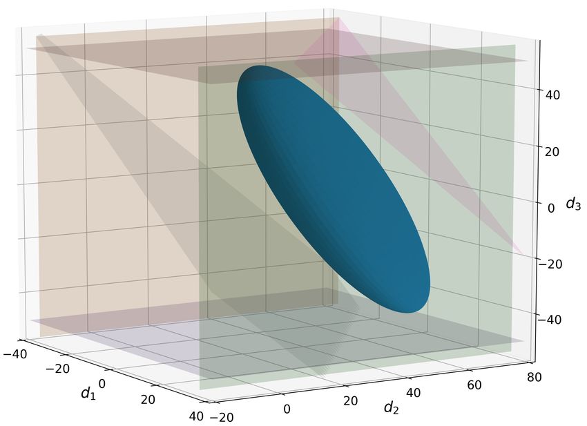
three dimensions. Figure 5 depicts the uncertainty sets of Table 5 with the center θ̄ f c . Here, it is clear
how intersecting the sets Tellip (δ) and Tbox (δ) with Rn+θ creates more exotic regions and this affects
the solution. Specifically, the intersected sets are scaled to a greater extent and they are limited by
different constraints (in comparison to their non-intersected counterparts). This again reflects that the
shape of T (δ) has a significant effect on the behavior of the flexibility index. Also, when Figure 5a is
juxtaposed with Figure 6b, it is apparent how the analytic center is more neutrally positioned between
the supplier capacity constraints (slanted planes) relative to the feasible center. This observation
13http://zavalab.engr.wisc.edu
explains why the flexibility is identical for the intersected and non-intersected sets.
(a) Tellip (δ) (b) Tellip+ (δ)
(c) Tbox (δ) (d) Tbox+ (δ)
Figure 5: A graphical representation of the optimized ellipsoidal and hyperbox uncertainty sets with
θ̄ = θ̄ f c corresponding to Design 1 of the 3-node network.
We now show Tellip (δ) can be used to conservatively approximate SF via the corresponding con-
fidence level α∗ and how correlation in θ affects indexes SF and F . Specifically, we consider the
combination of instances for β ∈ {−40, 0, 50} and θ̄ ∈ {θ̄ ac , θ̄ f c }. Table 6 summarizes the solutions
to these instances. Again, we observe that Fellip (and the corresponding confidence levels) mirror
the trends observed with SF at a significantly reduced computational cost. The correlation between
the random variables clearly has an impact on SF , which Fellip captures as well. On the other hand,
index Fbox does not capture this behavior since it cannot account for parameter correlation. Also, it
is apparent that the confidence levels associated with β = −40 provide a very tight lower bound for
SF , whereas the one associated with β = 50 has a much larger gap. This behavior illustrates how the
shape of the feasible region and that of the uncertainty set affect the tightness of the bound on SF
achieved by α∗ .
Figure 6 depicts the uncertainty sets corresponding to the results of Table 6. We note how the
14http://zavalab.engr.wisc.edu
Table 6: Results for Design 1 for various covariance values β.
Center β Fellip α∗ (%) SF -MC (%) Solution Time (s)
-40 15.31 99.84 99.99 0.18
analytic 0 8.93 96.97 99.71 0.21
50 4.31 77.02 96.22 0.18
-40 15.31 99.84 99.99 0.14
feasible 0 5.00 82.79 98.71 0.16
50 2.41 50.85 93.49 0.15
ellipsoidal set with β = −40 is able to scale to a greater extent relative to the set associated with
β = 50 because of its more favorable shape relative to the feasible region. This helps explain why α∗
is able to provide the tightest lower bound for SF with β = −40.
15http://zavalab.engr.wisc.edu
(a) β = −40 (b) β = 0
(c) β = 50
Figure 6: Ellipsoidal sets with θ̄ = θ̄ ac and different covariance values β (Design 1 of the three-node
network).
3.2.2 Design Comparison
To compare the three different designs described in Figure ??, we consider the results obtained with
θ̄ = θ̄ ac (the analytic center for Design 1) and β = 50. Table 7 summarizes these results. The results
indicate that Design 2 (which features decentralized suppliers) is less flexible than Design 1 (which
utilizes a centralized supplier scheme). This is surprising, since intuition suggests that decentral-
ization increases network flexibility. Our framework, however, shows that the converse is true in
this particular instance. This behavior results from the correlation structure of the random variables.
Furthermore, we observe that the arc added in Design 3 does not increase system flexibility (as one
might also intuitively expect). As we discuss next, this behavior results from non-obvious interplays
in the limiting constraints. This highlights how flexibility analysis can help guide system design.
16http://zavalab.engr.wisc.edu
Table 7: A summary of the flexibility index results using Fellip and Fbox to compare Designs 1, 2, and
3 of the three-node distribution network.
Fbox Fellip α∗ (%) SF -MC (%)
Design 1 0.578 4.310 77.02 96.22
Design 2 0.578 3.612 69.35 94.32
Design 3 0.578 4.310 77.02 96.20
3.2.3 Limiting Constraint Ranking
We use Design 1 to illustrate the limiting constraint ranking methodology described in Section 2.4,
letting θ̄ = θ̄ ac and β = 50 in conjunction with Tellip (δ). Table 8 summarizes the results. We observe
that the supplier capacity limits system flexibility the most. This explains why adding an arc in
Design 3 does not increase the flexibility of the network (i.e., the system is constrained by the inability
to supply power and not by the inability to transport power). As a result, one can improve flexibility
the most by increasing the supplier capacity (instead of adding an arc). Figure 7 depicts these results
by shading the limiting design components in accordance with their corresponding index Fellip . Here,
components are colored according to the value of Fellip corresponding to their rank level (a lower
value indicates that the component is more limiting). We thus see that supply is the most limiting
component, the left arc is the second most limiting component, and the right arc is the third most
limiting component.
Table 8: A summary of the constraint ranking results corresponding to Design 1 of the three-node
distribution network using the set Tellip (δ) with β = 50 and θ̄ = θ̄ ac .
Active Constraint Multipliers Fellip Flexibility Increase (%)
Rank 1 γ2U , γ2L 4.310 −
Rank 2 λU L
2:1 , λ2:1 15.312 255.3
Rank 3 λU L
2:3 , λ2:3 20.833 383.4
Figure 8 depicts the solutions corresponding to the results of Table 8. We see that the size of
Tellip (δ) significantly increases as limiting constraints are removed. In this study, we found that two
constraints simultaneously limit flexibility (corresponding to the maximum and minimum capaci-
ties of the limiting component). This indicates that the uncertainty set touches the boundary of the
feasible set at two locations.
17http://zavalab.engr.wisc.edu
Figure 7: Limiting components for three-node network. Colors are proportional to the corresponding
indexes Fellip (the smaller the value the most limiting the component is).
(a) Rank 1 (b) Rank 2
(c) Rank 3
Figure 8: Limiting components for Design 1 of three-node network using Tellip (δ) with θ̄ = θ̄ ac and
β = 50.
18http://zavalab.engr.wisc.edu
3.3 IEEE 14-Node Network
We now consider the IEEE 14-node power network, originally provided in Dabbagchi in [4]. The
system data is obtained from MATPOWER. This test case does not provide arc capacities so we en-
force aC = 100 for all the arcs. This base design is labeled Design 1 and a schematic of this system is
provided in Figure 9. Design 2 is obtained by removing the arc that connects node 2 to node 5 and by
removing the arc that connects node 9 to node 14. Design 3 uses a centralized power supply scheme,
this is accomplished by removing all of the suppliers except for the two located on nodes 1 and 2, by
increasing the capacity of each remaining supplier from 332 to 432 and from 140 to 340 respectively,
and by increasing the capacity of each arc to 200.
Figure 9: Schematic of the IEEE 14-node power system where the values sC are indicated and all the
values aC = 100.
This system is subjected to a total of 10 uncertainty disturbances (the network demands). The de-
mands are assumed to be θ ∼ N (θ̄, Vθ ), where θ̄ = θ̄ f c = (87.3, 50.0, 25.0, 28.8, 50.0, 25.0, 0, 0, 0, 0, 0)
and Vθ = 1200I. We select the sets Tbox+ (δ) and Tellip+ (δ) (the demands are nonnegative). Each
element of the hyperbox deviations ∆θ − , ∆θ + is set to 3σi = 103.92 (corresponding to θ̄ i ± 3σi con-
fidence bounds). Both of these sets are used to determine the flexibility index from Problem (1.7) for
each design. The stochastic flexibility index SF is computed using 1,000,000 MC samples.
Table 9 summarizes these design comparison results. Index SF shows that the flexibility of De-
sign 1 is worsened with the removal of the two arcs, whereas the centralized supply modification
improves flexibility. An observation is that Fellip+ mirrors the behavior SF at a much lower com-
putational cost. Specifically, Fellip+ required less than 20 seconds to compute while computing SF
using MC sampling required 13,030 seconds (3.6 hours). Index Fbox+ is not able to mirror the same
behavior (it does not indicate that Design 2 is less flexible than Design 1 as would be expected). This
analysis also shows that the higher capacity of the centralized supply scheme (Design 3) increases
system flexibility relative to Design 1, which again is counter-intuitive.
The limiting constraints of Design 1 are identified and ranked using Tellip+ (δ). The ranking results
are shown in Table 10. The capacity constraints corresponding to four of the five suppliers along with
three arc capacity constraints are identified as the most limiting ones. Again, this indicates that the
19http://zavalab.engr.wisc.edu
Table 9: Flexibility index results for various designs of IEEE-14 system.
Fbox+ Fellip+ SF -MC (%)
Design 1 0.327 10.594 97.84
Design 2 0.327 8.333 94.89
Design 3 0.404 12.244 99.91
uncertainty set touches the boundary of the feasible set at multiple points. We see that the next set
of constraints only have an index that is 15.6% larger meaning they are likely to also limit the system
flexibility to a certain extent. Subsequent sets have significantly increased flexibility indexes (up to
214% larger) and therefore have little effect on flexibility.
Table 10: Ranking of limiting constraints for IEEE-14 system.
Active Constraints Fellip+ Flexibility Increase (%) Solution Time (s)
Rank 1 λU U U U U U
1:2 , λ1:5 , λ6:11 , γ2 , γ3 , γ6 , γ8
U 10.594 − 16.61
Rank 2 λL L U L L L L
2:3 , λ2:5 , λ12:13 , γ1 , γ2 , γ3 , γ6 , γ8
L 12.243 15.6 3.76
Rank 3 λU U U U U U
2:3 , λ2:4 , λ3:4 , λ6:12 , λ6:13 , λ9:14 25.000 136.0 2.72
Rank 4 λU L U L L U
2:5 , λ5:6 , λ9:10 , λ9:14 , λ10:11 , γ1 33.333 214.6 0.14
Figure 10 highlights the limiting components of Design 1. The limiting constraints corresponding
to the active capacity constraints at each rank level are shaded according to the value of Fellip+ (the
lower the value, the most limiting the component is). We can see that the suppliers along with arcs
attached to such suppliers limit flexibility the most. The rest of the components follow non-intuitive
patterns, reflecting complex dependencies due to the network topology.
Figure 10: Limiting components for IEEE-14 power system. The colors are proportional to the corre-
sponding indexes Fellip+ (the smaller the value the most limiting the component is).
20http://zavalab.engr.wisc.edu
3.4 141-Node Network
Finally, we consider a 141-node power distribution network which corresponds to an urban area
in Caracas, Venezuela and was originally developed in [15]. The network data is extracted from
MATPOWER, but again no arc capacities are provided (we assume aC = 100). Figure 11 provides a
schematic of the network.
Figure 11: Schematic of the 141-node power distribution network.
This system is subjected to 84 uncertain disturbances (corresponding to the demands). The de-
mands are assumed to be θ ∼ N (θ̄, Vθ ), where θ̄ = θ̄ f c and Vθ = 100I. We use Tellip (δ) in combination
with Problem (1.7) to rank all the inequality constraints. This problem was solved 270 times while
iteratively removing the active constraints. We found that several solutions have the same value of
Fellip . Thus, the active constraints corresponding to solutions with equivalent Fellip values are com-
bined and assigned to the same ranks. A total of 44 rank levels were identified, the ranking data
corresponding to the first 30 levels is provided in Appendix A.
Figure 12 shows the limiting components corresponding to the 44 rank levels. We observe that the
supplier is the most limiting component along with the arcs that form the spanning tree of the net-
work (the path that connects all nodes in the network). The arcs become less relevant as they branch
out towards the network boundaries. We thus see that the flexibility framework reveals topological
limitations of the network. We also highlight that the flexibility index can be computed for this large
system in 20 seconds. In contrast, given the large number of random parameters, computing the SF
index using Monte Carlo sampling is impractical.
21http://zavalab.engr.wisc.edu
Figure 12: Limiting components for the 141-node power system. The colors are proportional to the
corresponding indexes Fellip (the smaller the value the most limiting the component is).
4 Conclusions and Future Work
We have presented a general framework to quantify and analyze system flexibility. This framework
provides several new features that include: generalizing uncertainty sets to consider compositions
of sets, finding a suitable nominal (center) point, and identifying and ranking limiting constraints.
We have demonstrated that this framework is often able to emulate the behavior of the rigorous
stochastic flexibility index problem at a significantly reduced computational cost. As part of future
work, we are interested in developing techniques to handle nonlinear and dynamical systems such
as reaction systems, heat exchanger networks, and transient power networks. We are also interested
in developing techniques that do not require the solution of bilevel optimization problems.
Acknowledgments
This work was supported by the U.S. Department of Energy under grant DE-SC0014114.
A Supplementary Material
The results for all of the instances discussed in Section 3.2 are summarized in Tables 11 and 12. Table
11 features the use of sets Tbox (δ) and Tellip (δ) for all designs, covariances, and centers considered
in the three-node network example. Table 12 features the use of the sets Tbox+ (δ) and Tellip+ (δ) for
22http://zavalab.engr.wisc.edu
the same system. Table 13 provides the first 30 rank levels corresponding to the results discussed in
Section 3.4 for the 141-node network.
Table 11: Results for three-node distribution network using sets Tbox (δ) and Tellip (δ).
Design Center β Fbox Time (s) Fellip Time (s) α∗ (%) SF -MC (%)
-40 0.578 0.03 15.31 0.18 99.84 99.99
analytic 0 0.578 0.03 8.93 0.21 96.97 99.71
1 50 0.578 0.03 4.31 0.18 77.02 96.22
-40 0.432 0.03 15.31 0.14 99.84 99.99
feasible 0 0.432 0.03 5.00 0.16 82.79 98.71
50 0.432 0.03 2.41 0.15 50.85 93.49
-40 0.578 0.08 3.61 0.21 69.35 96.82
analytic 0 0.578 0.08 3.61 0.23 69.35 96.56
2 50 0.578 0.08 3.61 0.19 69.35 94.32
-40 0.432 0.03 3.61 0.15 69.35 96.82
feasible 0 0.432 0.03 3.61 0.21 69.35 96.00
50 0.432 0.03 2.41 0.20 50.85 92.67
-40 0.578 0.04 37.81 0.20 100.00 100.00
analytic 0 0.578 0.04 8.93 0.16 96.97 99.72
3 50 0.578 0.04 4.31 0.16 77.02 96.20
-40 0.432 0.03 34.97 0.17 100.00 100.00
feasible 0 0.432 0.03 5.00 0.16 82.79 98.72
50 0.432 0.03 2.41 0.17 50.85 93.51
23http://zavalab.engr.wisc.edu
Table 12: Results for three-node distribution network using sets Tbox+ (δ) and Tellip+ (δ).
Design Center β Fbox+ Time (s) Fellip+ Time (s) SF -MC (%)
-40 0.578 0.04 18.38 0.14 100.00
analytic 0 0.578 0.04 8.93 0.10 99.44
1 50 0.578 0.04 4.31 0.13 94.33
-40 0.723 0.03 18.38 0.11 100.00
feasible 0 0.723 0.03 14.00 0.09 99.95
50 0.273 0.03 6.76 0.09 98.60
-40 0.578 0.04 26.46 0.18 100.00
analytic 0 0.578 0.04 8.82 0.16 99.34
2 50 0.578 0.04 4.31 0.13 94.23
-40 0.723 0.03 26.46 0.12 100.00
feasible 0 0.723 0.03 14.00 0.15 99.96
50 0.723 0.03 6.76 0.12 98.60
-40 0.578 0.03 45.38 0.20 100.00
analytic 0 0.578 0.03 8.93 0.11 99.45
3 50 0.578 0.03 4.31 0.06 94.34
-40 0.723 0.03 47.19 0.09 100.00
feasible 0 0.723 0.03 14.00 0.12 99.96
50 0.723 0.03 6.76 0.09 98.60
24http://zavalab.engr.wisc.edu
Table 13: Limiting constraints for 141-node network (determined using Tellip (δ)).
Active Constraint Multipliers Fellip Flexibility Increase (%) Solution Time (s)
Rank 1 λU1:2 , γ1
L 0.298 − 0.19
Rank 2 λU U U
2:3 , λ4:5 , λ3:4 0.705 151.9 2.43
Rank 3 λU5:6 1.110 273.0 4.35
Rank 4 λL5:6 1.365 358.8 4.98
Rank 5 λ4:5 , λ2:3 , λL
L L
3:4 1.767 493.8 6.00
Rank 6 U
λ6:7 2.034 583.5 1.62
Rank 7 λL6:7 2.223 646.9 2.20
Rank 8 λL1:2 2.679 800.0 4.13
Rank 9 λU6:37 2.770 830.8 5.89
Rank 10 λU7:8 2.986 903.2 7.99
Rank 11 λL,U
37:38 3.030 918.1 11.45
Rank 12 λL7:8 3.075 933.2 11.82
Rank 13 λL6:37 3.117 947.3 13.04
Rank 14 λL,U L,U
38:39 , λ8:9 3.125 949.9 25.67
Rank 15 λL,U L,U L,U
40:41 , λ39:40 , λ9:10 3.226 983.9 44.29
Rank 16 λL,U L,U
41:42 , λ10:11 3.333 1020 18.95
Rank 17 λL,U
11:12 3.448 1058.6 3.86
Rank 18 λL,U
12:13 3.571 1099.9 4.64
Rank 19 λL,U
13:14 3.846 1192.3 4.95
Rank 20 λL,U
14:15 4.000 1243.9 5.08
Rank 21 λ15:16 , λL,U
L,U
42:43 6.666 2139.9 14.41
Rank 22 λL,U
43:44 7.143 2299.9 6.78
Rank 23 λU7:88 7.579 2446.5 6.10
Rank 24 λL,U
16:17 , λ L,U L,U
42:54 , λ54:55 7.692 2484.5 11.51
Rank 25 λL7:88 7.806 2522.9 4.06
Rank 26 λL,U L,U
17:18 , λ88:89 8.333 2699.9 9.83
Rank 27 λL,U L,U
19:20 , λ18:19 9.091 2954.5 3.78
Rank 28 λL,U L,U L,U
20:21 , λ15:118 , λ118:119 10.000 3259.9 8.52
Rank 29 λL,U L,U L,U L,U
21:22 , λ22:23 , λ44:45 , λ45:46 11.111 3633.3 10.65
Rank 30 λL,U L,U L,U L,U
46:47 , λ55:60 , λ89:90 , λ90:91 12.500 4099.9 16.38
25http://zavalab.engr.wisc.edu
References
[1] V. Bansal, J. D. Perkins, and E. N. Pistikopoulos. Flexibility analysis and design of linear systems
by parametric programming. AIChE Journal, 46(2):335–354, 2000.
[2] S. Boyd and L. Vandenberghe. Convex optimization. Cambridge university press, 2004.
[3] D. A. Crowl and J. F. Louvar. Chemical process safety: fundamentals with applications. Pearson
Education, 2001.
[4] I. Dabbagchi. Ieee 14 bus power flow test case. American Electric Power System Golden CO, pages
557–576, 1962.
[5] I. Dunning, J. Huchette, and M. Lubin. Jump: A modeling language for mathematical optimiza-
tion. SIAM Review, 59(2):295–320, 2017.
[6] C. A. Floudas, Z. H. Gümüş, and M. G. Ierapetritou. Global optimization in design under uncer-
tainty: feasibility test and flexibility index problems. Industrial & Engineering Chemistry Research,
40(20):4267–4282, 2001.
[7] T. Gerstner and M. Griebel. Numerical integration using sparse grids. Numerical algorithms,
18(3-4):209, 1998.
[8] B. L. Gorissen, İ. Yanıkoğlu, and D. den Hertog. A practical guide to robust optimization. Omega,
53:124–137, 2015.
[9] J.-y. Gotoh and S. Uryasev. Two pairs of families of polyhedral norms versus `p -norms: proxim-
ity and applications in optimization. Mathematical Programming, 156(1-2):391–431, 2016.
[10] I. E. Grossmann, B. A. Calfa, and P. Garcia-Herreros. Evolution of concepts and models for
quantifying resiliency and flexibility of chemical processes. Computers & Chemical Engineering,
70:22–34, 2014.
[11] I. E. Grossmann and C. A. Floudas. Active constraint strategy for flexibility analysis in chemical
processes. Computers & Chemical Engineering, 11(6):675–693, 1987.
[12] I. E. Grossmann, K. P. Halemane, and R. E. Swaney. Optimization strategies for flexible chemical
processes. Computers & Chemical Engineering, 7(4):439–462, 1983.
[13] I. E. Grossmann and R. W. Sargent. Optimum design of multipurpose chemical plants. Industrial
& Engineering Chemistry Process Design and Development, 18(2):343–348, 1979.
[14] M. Jun and R. D’Andrea. Path planning for unmanned aerial vehicles in uncertain and ad-
versarial environments. In Cooperative control: models, applications and algorithms, pages 95–110.
Springer, 2003.
26http://zavalab.engr.wisc.edu
[15] H. Khodr, F. Olsina, P. De Oliveira-De Jesus, and J. Yusta. Maximum savings approach for loca-
tion and sizing of capacitors in distribution systems. Electric Power Systems Research, 78(7):1192–
1203, 2008.
[16] Z. Li, R. Ding, and C. A. Floudas. A comparative theoretical and computational study on ro-
bust counterpart optimization: I. robust linear optimization and robust mixed integer linear
optimization. Industrial & engineering chemistry research, 50(18):10567–10603, 2011.
[17] G. Papaefthymiou and D. Kurowicka. Using copulas for modeling stochastic dependence in
power system uncertainty analysis. IEEE Transactions on Power Systems, 24(1):40–49, 2009.
[18] K. Pavlikov and S. Uryasev. Cvar norm and applications in optimization. Optimization Letters,
8(7):1999–2020, 2014.
[19] E. Pistikopoulos and M. Ierapetritou. Novel approach for optimal process design under uncer-
tainty. Computers & Chemical Engineering, 19(10):1089–1110, 1995.
[20] E. Pistikopoulos and T. Mazzuchi. A novel flexibility analysis approach for processes with
stochastic parameters. Computers & Chemical Engineering, 14(9):991–1000, 1990.
[21] E. N. Pistikopoulos and I. E. Grossmann. Optimal retrofit design for improving process flexibil-
ity in linear systems. Computers & Chemical Engineering, 12(7):719–731, 1988.
[22] J. L. Pulsipher and V. M. Zavala. A mixed-integer conic programming formulation for comput-
ing the flexibility index under multivariate gaussian uncertainty. Computers & Chemical Engi-
neering, 2018.
[23] C. Robert and G. Casella. Monte Carlo statistical methods. Springer Science & Business Media,
2013.
[24] A. Shapiro. Sample average approximation. In Encyclopedia of Operations Research and Manage-
ment Science, pages 1350–1355. Springer, 2013.
[25] R. Smith. Chemical process: design and integration. John Wiley & Sons, 2005.
[26] D. A. Straub and I. E. Grossmann. Integrated stochastic metric of flexibility for systems with dis-
crete state and continuous parameter uncertainties. Computers & Chemical Engineering, 14(9):967–
985, 1990.
[27] R. E. Swaney and I. E. Grossmann. An index for operational flexibility in chemical process
design. part i: Formulation and theory. AIChE Journal, 31(4):621–630, 1985.
[28] A. Ulbig and G. Andersson. Analyzing operational flexibility of electric power systems. Inter-
national Journal of Electrical Power & Energy Systems, 72:155–164, 2015.
[29] J. Wang, J. Steiber, and B. Surampudi. Autonomous ground vehicle control system for high-
speed and safe operation. In 2008 American Control Conference, pages 218–223. IEEE, 2008.
27http://zavalab.engr.wisc.edu
[30] V. M. Zavala, K. Kim, M. Anitescu, and J. Birge. A stochastic electricity market clearing formu-
lation with consistent pricing properties. Operations Research, 65(3):557–576, 2017.
[31] Q. Zhang, I. E. Grossmann, and R. M. Lima. On the relation between flexibility analysis and
robust optimization for linear systems. AIChE Journal, 62(9):3109–3123, 2016.
[32] R. D. Zimmerman, C. E. Murillo-Sánchez, R. J. Thomas, et al. Matpower: Steady-state opera-
tions, planning, and analysis tools for power systems research and education. IEEE Transactions
on power systems, 26(1):12–19, 2011.
28You can also read