A Dream of Offspring: Two Decades of Intergenerational Welfare Mobility in Indonesia
←
→
Page content transcription
If your browser does not render page correctly, please read the page content below
A preliminary result
                      Do not quote any part of this article

A Dream of Offspring: Two Decades of Intergenerational Welfare
                     Mobility in Indonesia

   Teguh Dartanto1*, Canyon Keanu Can1 & Faizal Rahmanto Moeis1

Research Cluster on Poverty, Social Protection and Human Development,
Department of Economics, Faculty of Economics and Business, Universitas
                               Indonesia
        *Corresponding Author E-mail: teguh.dartanto@ui.ac.id

 Abstract. Economic mobility is key to achieving human progress and
 aspiration, as it determines the living standards of future generations.
 Taking advantage of the expenditure data in two decades of the
 Indonesian Family Life Survey (IFLS), we measure intergenerational
 expenditure mobility and use a novel Unconditional. We found that there
 has been a clear trend of welfare improvement across generations.
 Findings of high absolute and relative intergenerational mobility among the
 poorest and most vulnerable groups in Indonesia reflect the success of
 children in climbing above their parents on the economic ladder. The
 absolute intergenerational expenditure mobility is high and insensitive to
 age group among the poorest 40%. Moreover, the relative
 intergenerational mobility is also very high, with 9.29% of parents in the
 lowest quintile able to have their children climb to the highest quintile. OLS
 and UQR estimations show that the Intergenerational Elasticity of
 Expenditure (IGE) ranges from 0.162 to 0.192. The determinants of mobility
 are children’s years of schooling, age, gender of the household head, and
 asset ownerships of children. Timing of household split-off among parents
 and children have varying degrees of importance for absolute and relative
 mobility, with different impacts along the distribution. Hence, our findings
 suggest that an understanding of intergenerational expenditure mobility is
 critical in ensuring better living standards while maintaining less inequality.
 JEL Classification: J13, J62, I24
 Keywords: Intergenerational Mobility, Welfare Mobility, Quantile
 Regression, Children, Parent

                                                                              1
1. Introduction
The universal desire of parents to see their children achieve higher living
standards and the inherent desire of individuals themselves to climb higher up
the economic ladder has determined the rise and fall of civilizations. Thus,
intergenerational economic mobility (IGM) has long been, and continues to
be, a key element in human progress and aspiration. Indeed, the promise of a
better life is one which governments around the world pledge to their people.
Yet, recent evidence finds that, despite massive progress towards equal
access to opportunities, IGM trends have stalled since the 1960s, indicating
that societies have been less successful in generating greater and shared
prosperity (Narayan et al., 2018). A growing body of literature on IGM aims to
understand the dynamics and determinants of economic mobility, as they are
critical in reducing poverty, raising welfare and growth, and promoting
equality. A low absolute IGM signals a low improvement in living standards;
while a low relative IGM implies that privilege and poverty are highly persistent
across generations (Narayan et al., 2018, p.57).
One commonly used measure of IGM is the relative measure of
intergenerational elasticity (IGE), which measures the differences in outcomes
between children of low-income and high-income parents. However, research
on intergenerational mobility that focuses on measuring and analyzing
intergenerational elasticity has largely been conducted in developed
countries (Cervini-Plá, 2015; Chetty et al., 2017; Chetty, Hendren, Kline, & Saez,
2014; Chetty, Hendren, Kline, Saez, & Turner, 2014; Corak, 2013; Corak, Lindquist,
& Mazumder, 2014; Osterberg, 2000; Solon, 1999, 2002), and less in developing
countries in China, Africa and Latin America (Gong, Leigh, & Meng, 2012;
Lambert, Ravallion, & van de Walle, 2014; Narayan et al., 2018; Neidhöfer,
2019). This poses a challenge as most studies estimate IGE using the incomes
of both parents and offspring; in developing economies, income data is
relatively weak collected by statistical offices and also a less accurate
measure of welfare (Bavier, 2008; Fields, 1994; Meyer & Sullivan, 2003). Unlike in
developed countries, in developing countries consumption expenditure is
viewed as the preferred indicator in measuring welfare or living standards
because consumption can capture long run welfare levels than income
(World Bank., 2001). Consumption is less vulnerable to under-reporting bias as
income may fluctuate overtime due to some shocks or lifecycle income, while
consumption may smooth across seasons or years by saving or dissaving or by
other consumption smoothing mechanism. Consumption is more direct
measure of material well-being and a better basis for determining economic
status than is income (Bavier, 2008; Meyer & Sullivan, 2003).
Many studies have explored in the extent to which economic well-being
is transmitted across generations. Most of studies have focused on the
intergenerational income mobility or elasticity ( for example Chetty, Hendren,
Kline, & Saez, 2014; Corak, 2013; Gregg, Macmillan, & Vittori, 2019; Solon, 1999,
2002), where a relatively little attention on the intergenerational mobility in
consumption expenditure (Aughinbaugh, 2000; Bruze, 2018; Charles, Danziger,
Li, & Schoeni, 2014; Lambert et al., 2014; Waldkirch, Ng, & Cox, 2004).
2Consumption is more directly related to consumer’s utility than other indicators.
Moreover, the intergenerational expenditure correlation might also reflect a
particular preferences in the family utility function that might not associate
strongly in income or wealth correlation(Charles et al., 2014). Therefore, the
exploration on the intergenerational mobility in consumption expenditure may
reveal new insights about the transmission of well-being across generations.
Additionally, an understanding of the intergenerational persistence of
consumption allows for the analysis of long-run saving behaviors, consumption
smoothing, and wealth inequality (Bruze, 2018).
This paucity of literature is concerning, especially because
intergenerational mobility is heavily linked with the success of developing
economies. Therefore, taking advantage of the availability of long-term panel
data (the Indonesian Family Life Survey, or IFLS, that spans 21 years), we
examine the inequalities of opportunities that persist in a developing economy,
the channels through which they are perpetuated, and the characteristics
that allow low mobility to be broken. As a diverse country undergoing major
economic, social, environmental, and political upheavals, Indonesia's history
of intergenerational mobility can provide rich insight into how economic
mobility varies within developing countries.
Existing literature on Indonesia only explores intragenerational economic
mobility (Dartanto, Moeis, & Otsubo, 2019; Dartanto & Otsubo, 2016) and the
effects of child poverty on future labor outcomes (Rizky, Suryadarma, &
Suryahadi, 2019). The study of intergenerational mobility across generation in
Indonesia is fairly new. We then aim to close this research gap by using the IFLS
data set to explore the absolute and relative intergenerational expenditure
mobility. This study also introduces the novel method of unconditional quantile
regression (UQR), which has only recently been used in the canon of IGM
literature. The results guide policy makers to better design policies so that they
can foster greater equality of opportunities, reduce low mobility, and thereby
facilitate the fulfilment of people's aspirations.
This paper proceeds with a literature review discussing various measures
of intergenerational mobility, the findings of past research around the world,
and debates regarding appropriate methodologies. Then, the third section
presents an overview of the IFLS dataset is given, along with details on how
classifications, thresholds, and percentiles are constructed. The fourth section
follows with an exploration of changes and trends in living standards in
Indonesia. The fifth section describes the research methodologies employed
to delve further into the data, and the results are analyzed in the sixth section.
The paper concludes by summarizing our main findings and considering their
policy implications.
2. Literature Review on Intergenerational Mobility
2.1 Concept of Absolute and Relative Intergenerational Mobility
Economic mobility itself is the ability of individuals, families, and groups
to improve their economic status. The focus is often on incomes as a measure
of living standards, and strands of literature in economic mobility study
3intragenerational (the ability of individuals to climb the economic ladder within
their own lifetimes) and intergenerational (the ability of children to climb
above their parents in the economic ladder) mobility.
The general convention in estimating intergenerational mobility is to
distinguish between relative and absolute measures; measures of mobility can
also differ by the outcome variable of interest (e.g. educational mobility,
income mobility, consumption mobility, etc.) and by how outcome variables
are distributed (e.g. continuously or discretely). When variables are discretely
distributed, individuals are often grouped into quartiles or quintiles and the
probabilities of transition between quantiles is a measure of relative mobility
that can be organized into a transition matrix (Narayan et al., 2018).
Relative mobility measures the extent to which children’s outcomes
depend on their parents’ outcomes. The greater the dependence, or the
greater the intergenerational persistence (IGP) in outcomes, the less
intergenerational mobility there is. Conversely, greater independence implies
greater intergenerational mobility as it indicates that the fate of children is less
constrained by the fate of their parents. Widely used measures of relative
mobility include intergenerational elasticity, which is obtained by regressing
log child outcomes with log parent outcomes, and the rank-rank slope, which
measures the relationship between children’s positions and their parents’
positions on the income distribution (Chetty, Hendren, Kline, & Saez, 2014;
Narayan et al., 2018). However, both measures possess the drawback that they
are unable to differentiate between upward and downward mobility, are
informative of non-linearities in mobility (e.g. whether mobility is greater or
lower in certain parts of the distribution), and, as will be further discussed later,
can also be sensitive to how outcomes are measured and distributions are
varied (Corak et al., 2014; Gregg et al., 2019). Thus, Corak et al., (2014) utilizes
a directional rank mobility measure which resolves, to an extent, the first two
drawbacks, and Gregg et al., (2019) applies an unconditional quantile
regression to resolve the latter drawback.
Meanwhile, absolute mobility measures the extent to which children’s
outcomes differ from their parents. There are three widely used measures of
relative mobility. Absolute upward mobility measures the mean rank (or
percentile in the national distribution) of children whose parents are located
at a certain percentile in the national distribution. In the context of income
mobility, Chetty, Hendren, Kline, & Saez, (2014) estimates the mean rank of
children whose parents are at the 25th percentile in the national income
distribution. Although this measure is analogous of the rank-rank slope at the
national level, when analysis is conducted at smaller levels, the measure
becomes an absolute measure as incomes in individual areas have little effect
on the national distribution (Chetty, Hendren, Kline, & Saez, 2014). The second
measure of absolute mobility estimates the probability of rising from the bottom
quintile to the top quintile, and the third measure estimates the probability that
a child will exceed a certain threshold (e.g. poverty line) given that their
parent’s income is at a certain percentile (Chetty, Hendren, Kline, & Saez,
2014).
4Absolute mobility is important as, ceteris paribus, it allows for Pareto
improvements in welfare that do not come at the expense of other groups in
society. It is required for the improvement of living standards because it
measures the ability of societies to expand the economic pie so that different
groups do not compete for the same slice of a stagnant or shrinking pie and
social cohesion does not deteriorate (Chetty, Hendren, Kline, & Saez, 2014;
Narayan et al., 2018). Meanwhile, rising relative intergenerational mobility does
not necessarily indicate that the living standards of the poor are improving; it
may indicate that the rich are doing less well than they did in the past.
However, even such trends in mobility are important; an absence of relative
mobility represents intergenerational persistence of inequalities of opportunity,
wasted human potential, and misallocation of resources. Thus, both measures
of intergenerational mobility are necessary for economic progress and for the
sustainability of the social contract that addresses the aspirations of society
(Narayan et al., 2018).
Studies using both relative and absolute measures of mobility find a
wealth of diversity in intergenerational performance and its determinants.
Chetty, Hendren, Kline, & Saez, (2014) finds that IGM in income varies widely
in the United States, with high mobility areas being characterized by less
residential segregation, lower inequality, better primary schools, greater social
capital, and greater family stability; significant childhood exposure effects to
neighborhood characteristics are further found in (Chetty & Hendren, 2018). In
the United Kingdom, childhood exposure effects are also significant, but in
terms of early skills, education, and early labor market attachment, as these
variables mitigate, albeit not fully, the strong intergenerational persistence in
the country (Gregg et al., 2019). A comparison of IGM in income among
several developed economies finds that Britain’s exceeds Spain’s, and Spain’s
is similar to France’s but exceeds Italy’s and the United States (Cervini-Plá, 2015).
When direction of mobility is considered, it is found that Canada possesses
higher downward mobility than Sweden and the United States, while upward
mobility is similar in the three countries (Corak et al., 2014). In all countries, the
extent of IGM and its determinants are nonlinear across the distribution; for
example, returns to education are higher at the top of the income distribution
while youth unemployment most adversely impacts the mobility of those at the
bottom of the distribution (Gregg et al., 2019)(Gregg et al., 2019). These
nonlinearities may reflect the availability of egalitarian public facilities and
redistributive welfare programs (Torche, 2015).
The scope of IGM may be broadened by extending analyses beyond
earnings and income to include other outcome variables such as educational
mobility, occupational status mobility, class mobility, and gender-based
mobility. Narayan et al. (2018) provides a highly comprehensive analysis of
intergenerational educational mobility across the world, as extended datasets
on education are widespread and comparable, allowing educational mobility
to be uniquely studied at the global level. Moreover, Intergenerational
persistence is stronger in developing economies, where the education of
5grandparents influences the educational attainment of individuals to a greater
extent than that found in richer economies (Narayan et al., 2018).
2.2 Intergenerational Expenditure (Consumption) Mobility
It is, however, evident that a majority of these studies have been
conducted in developed economies. Yet, Narayan et al. (2018) show that IGM
trends in developing economies are different to those observed in more
developed ones. We now turn to another novel approach to mobility is to
analyze mobility in consumption or expenditure rather than income. If
measurements of IGM aim to measure how living standards of children are
affected by their parents’ living standards, then consumption or expenditure
would be a better indicator of material welfare than income (Bruze, 2018;
Deaton & Zaidi, 2002; Meyer & Sullivan, 2003). A small number of studies have
used consumption as a proxy for IGM, and although studies on United States
data reach conflicting results, Bruze (2018) finds that, in Denmark,
intergenerational elasticity of consumption significantly exceeds both
intergenerational elasticity of disposable income and intergenerational
elasticity of earnings. Such findings indicate that calculating intergenerational
persistence using intergenerational elasticity of earnings (the lowest among
the three measures) can greatly underestimate the persistence of living
standards and therefore overestimate economic mobility.
The intergenerational mobility of consumption approach is also
particularly relevant in the context of understanding IGM in developing
countries, as income datasets may not be available or are poorly collected in
many developing countries, hence making income a less accurate measure
of welfare. Although lengthy expenditure datasets that are sufficient to
describe intergenerational mobility are rare for developing economies, those
that do exist can provide unique insight into the extent of economic mobility
found in poor, primarily rural, and largely agricultural societies, many of which
are struggling to raise their standards of living. Lambert et al., (2014) uses
expenditure data on Senegal to understand the dynamics of intergenerational
mobility and interpersonal inequality, and they discover that mobility is higher
when greater economic activity of women and a shift away from farming
sectors are observed. They also discover that inheritance of land and housing
have little effect on children’s consumption and on inequality, whereas
inheritance of non-land assets, parental education and occupation, and
parental choices about children’s schooling play more significant roles in
raising the child’s welfare as an adult. These positive intergenerational effects
were found to be stronger from the mother’s side.
While debates on the efficacy of absolute versus relative measures have
long existed in estimating intergenerational mobility, there has recently arisen
debates regarding the use of conditional versus unconditional measures
(Gregg et al., 2019). The relative and absolute measures discussed above are
the result of conditional regressions and are therefore subject to greater
sensitivity towards the distribution of variables. The measures are conditional
because they rely on the child’s conditional income distribution in order to
6obtain a conclusion about economic mobility. Conditionality not ideal
because the pre-regression rank order of children’s earnings is not the same as
that for the post-regression residuals, causing unclear interpretation of
coefficients (Firpo, Fortin, & Lemieux, 2009; Gregg et al., 2019).
Also, conditionality creates difficulties in adding covariates, as
conditional quantiles vary across specifications. For example, the distribution
for someone at the 10th percentile of the wage distribution of university
graduates may not be the same as the distribution for someone at the 10th
percentile of the wage distribution of all workers. Therefore, unlike OLS
estimates, conditional quantile regression (CQR) estimates do not allow us to
retrieve the marginal impact of a specific variable (e.g. university education)
on the unconditional quantile of the dependent variable. They only allow us to
conclude what the distribution (e.g. the expected value or mean) of the
child’s outcome variable will be (Firpo et al., 2009; Gregg et al., 2019).
3. Measuring Intergenerational Mobility: Methods and Dataset
3.1 Absolute Mobility: Measurement and Determinants
We now turn to empirical estimates of absolute and relative mobility
using consumption expenditure data. As previously noted, expenditure or
consumption can be a more accurate representation of living standards,
particularly in developing economies (Aughinbaugh, 2000; Bruze, 2018;
Charles et al., 2014; Lambert et al., 2014). Following Chetty et al., (2017) but
modifying for our use of expenditure instead of earnings to measure mobility,
we define absolute mobility, !" , as the percentage of children in cohort c that
&
spend weekly more than their parents. Let $%" denote the expenditure
'
(capita/month) of child i in cohort c, $%" denote the expenditure
(capita/month) of their parent, and (" be the number of children in the cohort.
We use the consumer price index to convert the nominal value of expenditure
into the real term of expenditure per-capita. During two decades, the
consumer price index had jumped from 100 in 1993 becoming 763 in 2014. Then,
absolute mobility is defined as:
1
!" = &
+ 1{ $%" ≥ $%"' }
("
%
Children and parents are then divided into two cohorts, based on whether
they are aged above or below 40 years old. The children of ages 20 to 40 years
old in 2013 with parents of ages 20 to 40 years old in 1993 are grouped into one
cohort, and children of ages 40 and above in 2014 with parents of ages 40 and
above in 1993 are grouped into another cohort. The expenditures of children
and parents within cohorts are compared in order to obtain absolute mobility.
Although grouping different ages into one cohort and distinguishing cohorts
using the age of 40 as a threshold may introduce biases such as the life-cycle
bias, we find that such a division results in the most consistent estimates.
Moreover, it is intuitive to divide the sample using such a threshold because we
observe divergent trends in mobility between the two cohorts.
7Logit models are also regressed in order to identify the marginal effects
of parents’ conditions in 1993 and their children’s conditions in 2014 on
intergenerational mobility. The first model includes only variables describing
parents’ conditions in 1993, while the second model also includes variables
describing children’s conditions in 2014. Two variants of each model is
regressed: one showing the marginal effects for when the expenditure
distribution is grouped into deciles, and another for when it is grouped into
vigintiles.
& ' '
$%" = / 0 + 230 4%3 + ⋯ + 260 4%6 + 7%0 4%6
&
+ ⋯ + 7%0 4%6
&
+ 8%
&
where, $%" is the discrete variable of the absolute mobility of children in
which 1 represents that children has a higher or equal rank than their parents
'
and 0 represents that children has a lower rank than their parents. 4%9& :4%9 ;
denotes child (parent) i's j-th characteristic of interest (e.g. child i's level of
education) whereas 290 & 790 denote the returns or impacts of those
characteristics at each quintile s across the distribution (Gregg et al., 2019).
3.2 Measuring Relative Mobility and Unconditional Quantile Regression
Relative mobility is then estimated as the intergenerational elasticity, rank-rank
slope, and directional rank mobility (Chetty, Hendren, Kline, & Saez, 2014;
Corak, 2013; Corak et al., 2014; Gregg et al., 2019). The intergenerational
expenditure elasticity is obtained by regressing log child income (logYi) on log
parent income (logXi), whereas the rank-rank slope is obtained by calculating
the correlation between the child’s position (quantile rank, represented by Ri)
on the expenditure distribution and the parent’s position (quantile rank,
represented by Pi) on the distribution. The rank-rank slope can be obtained by
regressing Ri on Pi. Mathematically, the regression coefficients may be
represented as (Chetty et al., 2914):
CB MN(HEIK% )
=>? = @AB = DEFF(HEI4% , HEIK% )
CA MN(HEI4% )
OPQR SHETU = @VW = DEFF(X% , O% )
When the elasticity and slope are higher, intergenerational expenditure
mobility is lower, because the two measures represent the intergenerational
persistence in expenditure. The elasticity and slope differ only to the extent that
inequality or the standard deviation of expenditures is higher across
generations, with rising inequalities leading to a greater intergenerational
elasticity (Chetty et al., 2014).
Finally, in addition to the conditional measures above, we also conduct
unconditional quantile regressions in order to identify covariates which
influence intergenerational expenditure mobility. Ranking the children into
quintiles, we apply the re-centered influence function (RIF) technique as found
in Firpo et al. (2009) and Gregg et al. (2019):
&
O=Y:$%" ; [0 ; = / 0 + \ "0 $%"' + 230 4%3
' '
+ ⋯ + 260 4%6 + 7%0 4%6
&
+ ⋯ + 7%0 4%6
&
+ 8%
8using UQR at different quintiles [0 where s takes the values of 0.2, 0.4, 0.6 and
0.8. The estimate \] "0 is the association between parent and child expenditures,
conditional on all other variables. 4%9& :4%9' ; denotes child (parent) i's j-th
characteristic of interest (e.g. child i's level of education) whereas 290 & 790
denote the returns or impacts of those characteristics at each quintile s across
the distribution (Gregg et al., 2019). As discussed above, the use of the UQR
and RIF approach allows for straightforward interpretation of the marginal
effects of each variable, but with modifications for discrete variables.
In estimating our RIF, we divide variables into two groups: the condition
of parents in 1993, and the condition of children in 2014. Both groups of
variables include parents’ and children’s respective age, gender of the
household head, years of schooling, location of the household, and value of
asset ownership. Moreover, in order to add nuance to the condition of children
in 2014, we also include as a variable the year in which children split from their
parents’ households to create a new household of their own.
The use of unconditional quantile regression (UQR) allows for consistent
interpretation of additional covariates in the model and for between-group
comparisons because quantile distributions no longer vary across
specifications. Coefficients for continuous variables such as income may be
interpreted in the same way as OLS estimates, although for discrete variables
such as years of schooling, the UQR coefficient reflects the impact of an
increase in the proportion of schooling in the quantile (Firpo et al., 2009; Gregg
et al., 2019). Unconditional quantiles are constructed using a re-centered
influence function (RIF) that allows mobility to be estimated more reliably at
different parts of the distribution and for additional variables to be added
consecutively to the regression (Firpo et al., 2009). CQR and UQR estimates can
differ greatly from each other, and their divergence can also provide insight
into mobility dynamics.
4. Indonesia Family Life Survey (IFLS) Dataset and Overview of
Intergenerational Mobility
4.1 Overview of the Indonesia Family Life Survey (IFLS) Dataset
We use mainly the 1993 and 2014 waves of the IFLS to measure
intergenerational expenditure mobility in Indonesia throughout the last two
decades. The IFLS is a longitudinal survey, in which the sample of households in
subsequent waves are primarily determined by the household sample in the
first wave. The first wave, or the IFLS1 was conducted in 1993 following the
sample frame of the national socio-economic survey (SUSENAS). The IFLS1 used
a sampling scheme that stratifies by provinces, then conducts random
sampling within provinces. The sampled provinces were the thirteen major
provinces of Indonesia where approximately 83% of the population resided.1
The IFLS dataset provides uniquely rich detail of households’ demographics,
1
The original sample represented around 83% of the population, but recent samples
cannot guarantee a similar representation rate due to attrition, split-off households,
and migration.
9socioeconomic characteristics, consumption behaviours, health conditions,
and access to community facilities and social safety nets (see Frankenberg
and Karoly 1995 and Frankenberg and Thomas 2000).
The IFLS1 interviewed 7,224 households, while the IFLS2 in 1997
interviewed 7,619 households. The sample increased as split-off households
created when children began their own households were also surveyed in
IFLS2; around 11.5% of IFLS2 households are split-off households. In the IFLS3
conducted in 2000, approximately 35% of the households surveyed were split-
off households, including those who split in and after 1997. The IFLS4
interviewed 13,535 households; the IFLS5 interviewed 16,930 households of
which 5,053 were original IFLS1 households, 7,862 were old split-off households
from IFLS2, 3, and 4, and 4105 were new split-off households. However, despite
the richness of the data, we focus only the original households of IFLS1 because
it is those households which always appear in every wave of the survey
throughout the last two decades.
The attrition rate is usually the Achilles heel of longitudinal studies. Yet,
unlike many longitudinal household surveys in many developing countries
where follow-up surveys explicitly target only the subset of respondents
remaining in their baseline location, the IFLS aims to minimize attrition by
constantly tracking respondents who move to other locations. Thomas et al.
(2001) show that the attrition between the baseline and second follow up is
only 5%. At least one member of every 20-target households was re-contacted
in each of the three follow-up surveys (Thomas et al., 2012; Dartanto et al.,
2019). The critical feature behind successful tracking is to provide interviewers
and trackers with detailed information on a wide range of the individual,
household, and family attributes of respondents (Thomas et al., 2012).
Having merged the IFLS1 and IFLS5, we calculated an attrition rate of
only 16.33%. 2 As our focus is not only on intergenerational welfare mobility
throughout the two decades of survey data but also on its determinants, we
create a combined dataset of all household characteristics of parent
households in IFLS1 and their children’s households in IFLS5 for econometric
estimations. Among the characteristics we include are the education, gender,
age, expenditure pattern, and asset ownership.
4.2 Overview of Absolute and Relative Intergenerational Mobility
Figure 1 shows the density of expenditure per capita. In 1993, the
expenditure was highly dense between IDR10,000-50,000 per capita per month.
However, in recent years, the density in real terms has flattened out, being
more dispersed, which may be signal lower equality across generations.
Meanwhile, Figure 2 shows that absolute mobility declines as parent
expenditure increases, with absolute mobility being highest for the poorest and
most vulnerable groups at the bottom of the distribution. Moreover, for those
2This attrition rate is the household attrition rate, not individual attrition rate. It is
possible that the individual attrition rate is much higher than that of households.
10whose expenditures are in the bottom 40% of the distribution, absolute mobility
is not sensitive to the age at which the child’s and parents’ expenditures are
measured. This is desirable, because regardless of the stage of life of parents
or children, the most vulnerable children are able to consume more than their
parents, therefore implying greater chances for those children to achieve
better living standards than their parents.
Yet, as we move up the expenditure distribution, we find that absolute
mobility becomes sensitive to the age at which it is measured, with
intergenerational expenditure mobility being greater for those in the 20- to 40-
year-old cohort than those in the 40-and-above cohort. The factors influencing
this mobility gap among the non-poor are left to future work, as we are largely
concerned with intergenerational mobility among the poor, for whom moving
up the income ladder has the highest stakes. Still, we explore some of the
dynamics behind the differences in the following section, where we examine
in greater detail some of the determinants behind absolute and relative
mobility, one of which being the age at which children split off from their
parents’ households to begin their own household.
Figure 1. Distribution of Expenditure between Parent and Children
.00002
.000015
Density
.00001
5.000e-06
0
0 500000 1000000 1500000 2000000 2500000
Monthly HH per capita expenditure
Kernel Density Parent Expenditure in 1993
Kernel Density Children Expenditure in 2014
kernel = epanechnikov, bandwidth = 4.3e+03
11Figure 2. Absolute Mobility Based on Age Cohort: Decile
% of Children Expenditure (per capit/month) more than their Parents 100
90
80
70
60
50
40
30
20
10
0
1 2 3 4 5 6 7 8 9 10
Parent Expenditure Decile (per capita/month) in 1993
[20-40) 40+ All
Source: Authors’ estimation
Figure 3. Absolute Mobility Based on Age Cohort: Vigintile
100
% of Children Expenditure (per capita/month) more than their Parents
90
80
70
60
50
40
30
20
10
0
1 2 3 4 5 6 7 8 9 10 11 12 13 14 15 16 17 18 19 20
Parent Expenditure Vigintile (per capita/month) in 1993
[20-40) 40+ All Age
Source: Authors’ estimation
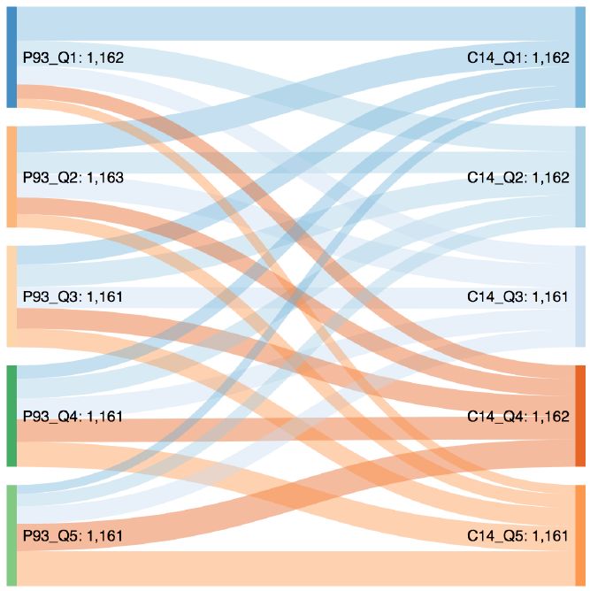
12Figure 4 illustrates the long run transition of intergenerational
consumption mobility between parent and children. Around 9.19% of children
from the 1st quintile of parents can climb up the economic ladder into the 5th
quintile income during two decades, while 33.65% of children of the 1st quintile
remained at the same quintile. However, only 35% of children from the richest
expenditure group (quintile 5) can maintained their consumption level as
same as their parents. Most of them dropped to the lower expenditure group.
Surprisingly, around 9% of children from the richest expenditure group became
the poorest group. These figures verify that the individual in Indonesia is very
mobile both upward and downward mobility.
Figure 4. Relative Mobility between Quintile: Parent vs. Children
Source: Authors’ estimation
135. Analysis of Results
5.1 Absolute Intergenerational Mobility
Having observed the general trends in intergenerational mobility, we first
turn to our logistic regression which attempts to identify the marginal effects of
various variables on the probability of absolute upward mobility or,
equivalently, of a child’s expenditures weakly exceeding their parents’
expenditures. Results for when the distribution is divided into deciles and into
vigintiles are similar for almost all variables. When only the characteristics of
parents are considered, we find that parents living in urban areas and an
increase in parents’ years of schooling reduces the probability of absolute
mobility. This is natural as the more educated parents are, the higher their
expenditures are likely to be, thereby reducing the room that children have to
increase expenditures beyond their parents’ levels. Similarly, the older parents
are in 1993, the less chance for absolute upward mobility in children, which
may be linked with the ability for parents to provide for themselves and or their
children.
Meanwhile, when characteristics of children are also considered, the
effect of the age of parents in 1993 reverses and becomes insignificant. The
value of parents’ asset ownership becomes a negative and significant
determinant of chances for absolute upward mobility, and the age of the child
themselves also negatively impacts chances for mobility. Chances of upward
mobility are further negatively influenced by the year in which children split
away from their parents’ households to create their own households. However,
the child’s own years of schooling, residence in urban areas, and asset
ownership increases the probability of greater expenditures. Together, these
findings reflect intergenerational persistence because parents’ conditions
diminishes chances for mobility, but with the persistence being weakened due
to the child’s ability to influence their absolute outcomes through their own
attributes.
Yet, these results must be treated with caution, as the conditionality of
the measure on the distributions within each quantile can result in inconsistent
estimates and misleading interpretations. Additionally, the marginal effects
provide no clarity on the non-linearities of the effects along the expenditure
distribution, therefore limiting their insight and usefulness. Therefore, we now
turn to our unconditional quantile regression results.
We find that although value of parents’ asset ownership influences
absolute mobility, it does not influence relative mobility. The negative effects
of parents’ years of schooling on absolute mobility is contradicted by its
positive effects on relative mobility. Still, the effects of the child’s age, years of
schooling, value of asset ownership, and timing of household split-off remain
similar for absolute and relative mobility. The differences between the results
can provide policy guidance for which aspects of individuals and households
to target in order to achieve both an increase in living standards and a
reduction in inequality.
14Table 1. Results of Logistic Regression
VARIABLES Limited Dependent Variable:
1= Children expenditure weakly more than Parents , 0= Others
Absolute Mobility (Group 10) Absolute Mobility (Group 20)
Marg. Effect Marg. Effect Marg. Effect Marg. Effect
Parent Condition 1993
Age (years) -0.006** 0.004 -0.007*** 0.005
(0.003) (0.003) (0.003) (0.003)
Sex of Household Head 0.159* 0.103 0.124 0.055
(1=male; 0=other) (0.096) (0.100) (0.096) (0.100)
Years of Schooling -0.022*** -0.036*** -0.027*** -0.040***
(0.007) (0.008) (0.007) (0.008)
Location -0.395*** -0.490*** -0.402*** -0.504***
(1=urban, 0=other) (0.058) (0.066) (0.058) (0.066)
Value of Asset Ownership -0.006 -0.007* -0.008** -0.010**
(log)
(0.004) (0.004) (0.004) (0.004)
Children Condition in 2014
Age (years) -0.019*** -0.024***
(0.005) (0.006)
Sex of Household Head 0.045 0.074
(1=male; 0=other) (0.054) (0.054)
Years of Schooling 0.021*** 0.019**
(0.008) (0.008)
Location 0.255*** 0.299***
(1=urban, 0=other) (0.066) (0.065)
Asset Ownership (log) 0.009** 0.012***
(0.004) (0.004)
Offspring split in 1993 -0.147 -0.177
(1=1997; 0=others) (0.121) (0.120)
Offspring split in 2000 -0.123 -0.166**
(1=2000; 0=others) (0.083) (0.083)
Offspring split in 2007 -0.165** -0.180***
(1=2007; 0=others) (0.067) (0.066)
(base offspring in 2014)
Constant 0.718*** 0.720*** 0.695*** 0.737***
(0.154) (0.202) (0.153) (0.202)
Observations 5,808 5,808 5,808 5,808
dy/dx is for discrete change of dummy variable from 0 to 1
Robust standard errors in parentheses
*** pearnings and education in Indonesia and other economies, the different
estimates for mobility that intergenerational expenditures provide may
indicate that children’s living standards are less constrained by their parents’
than previously thought.
Both the IGE and the rank-rank slope for intergenerational expenditures
fall but remain significant when other covariates are considered, with varying
effects at each quantile of children’s expenditures. Based on the IGE resulted
from both OLS and UQR estimations, we show that the IGM in Indonesia ranges
from 0.80 to 0.83 :1 − \] "0 ;, while from the rank-rank regressions, the IGM ranges
from 0.75 to 0.84. These mean that individual in Indonesia is very mobile in
which children from a very poor family can easily climb up to the upper class.
Unconditional quantile regression results from the IGE and rank-rank slope
approach also generally concur with each other in terms of the variables that
are significant in determining a child’s expenditure in 2014, although
coefficients of the two approaches differ due to the different nature of the
variables involved. However, as previously discussed, some results from the
UQRs contradict the estimates obtained through the previous logit regression,
especially as we find that the logit marginal effects to do not hold true at
certain areas of the expenditure distribution.
All UQRs indicate the importance of parents’ expenditures in
determining their child’s expenditures across the income distribution, and
agree that intergenerational persistence or correlation in expenditures is lower
in the first quintile. This is desirable in the effort to reduce inequality, as it implies
that the living standards of the very poor are relatively more mobile than their
counterparts. The greater mobility among the very poor may also be reflected
in our finding that the proportion of parents with greater years of schooling
significantly and positively affects children’s expenditures in all quintiles except
the bottom quintile. Moreover, the proportion of children with greater years of
schooling significantly and positively affects their expenditures in all quintiles
including the bottom quintile, indicating that, at least for the poorest group,
children are able to improve their living standards through their own efforts in
spite of their parents’ conditions.
16Table 2. Estimation Results of OLS and Unconditional Quantile Regression: Expenditure
VARIABLES Dependent Variable: Children Expenditure (per capita/month) (log) in 2014
OLS Unconditional Quantile Regression (RIF)
Model 1 Model 2 Model 3 20th 40th 60th 80th
Parent expenditure 1993 0.303*** 0.226*** 0.165*** 0.166*** 0.153*** 0.180*** 0.192***
(capita/month) (log) (0.012) (0.013) (0.013) (0.017) (0.015) (0.017) (0.023)
Parent Condition 1993
Age (Years) -0.004*** -0.000 -0.003** -0.000 0.001 0.001
(0.001) (0.001) (0.001) (0.001) (0.001) (0.002)
Sex of Household Head -0.043 -0.049* -0.044 0.018 -0.035 -0.102**
(1=male; 0=other) (0.029) (0.028) (0.039) (0.034) (0.040) (0.052)
Years of Schooling 0.026*** 0.010*** -0.003 0.006** 0.014*** 0.023***
(0.002) (0.002) (0.003) (0.003) (0.003) (0.005)
Location 0.074*** -0.033* 0.012 -0.009 -0.036 -0.100***
(1=urban; 0=other) (0.019) (0.020) (0.025) (0.023) (0.027) (0.037)
Value of Asset Ownership (log) 0.002 0.001 -0.000 -0.000 0.002 0.001
(0.001) (0.001) (0.002) (0.001) (0.002) (0.002)
Children condition 2014
Age (Years) -0.007*** -0.001 -0.002 -0.005** -0.013***
(0.002) (0.002) (0.002) (0.002) (0.003)
Sex of Household Head 0.064*** 0.017 0.020 0.051** 0.137***
(1=male; 0=other) (0.016) (0.021) (0.018) (0.021) (0.029)
Years of Schooling 0.039*** 0.034*** 0.033*** 0.040*** 0.046***
(0.003) (0.003) (0.003) (0.003) (0.004)
Location 0.249*** 0.197*** 0.221*** 0.293*** 0.328***
(1=urban; 0=other) (0.020) (0.026) (0.023) (0.026) (0.034)
Asset Ownership (log) 0.007*** 0.006*** 0.006*** 0.008*** 0.008***
(0.001) (0.001) (0.001) (0.001) (0.002)
Offspring split in 1997 0.058* 0.067 0.065 0.091* 0.018
(1= 1997; 0=others) (0.034) (0.045) (0.041) (0.049) (0.063)
Offspring split in 2000 -0.049** -0.003 -0.037 -0.070** -0.106**
(1= 2000; 0=others) (0.024) (0.033) (0.028) (0.032) (0.041)
Offspring split in 2007 -0.051*** -0.014 -0.035 -0.051* -0.092***
(1= 2007; 0=others) (0.020) (0.026) (0.023) (0.026) (0.035)
(base offspring in 2014)
Constant 8.566*** 9.414*** 9.650*** 9.159*** 9.475*** 9.417*** 9.910***
(0.124) (0.139) (0.135) (0.174) (0.152) (0.181) (0.246)
Observations 5,808 5,808 5,808 5,808 5,808 5,808 5,808
R-squared 0.104 0.137 0.219 0.095 0.133 0.159 0.129
Robust standard errors in parentheses; *** pTable 3. Estimation Results of OLS and Unconditional Quantile Regression: Percentile Rank
Dependent Variable: Children Rank Percentile in 2014
VARIABLES OLS Unconditional Quantile Regression (RIF)
Model 1 Model 2 Model 3 20th 40th 60th 80th
Parent Rank Percentile in 1993 0.322*** 0.239*** 0.175*** 0.187*** 0.246*** 0.252*** 0.162***
(0.012) (0.014) (0.014) (0.020) (0.024) (0.024) (0.020)
Parent Condition in 1993
Age (years) -0.161*** -0.022 -0.130** -0.014 0.005 0.036
(0.033) (0.041) (0.063) (0.075) (0.071) (0.058)
Sex of Household Head -1.502 -1.458 -1.144 1.448 -1.551 -3.621*
(1=male; 0=other) (1.287) (1.256) (1.829) (2.262) (2.263) (1.858)
Years of Schooling 1.106*** 0.383*** -0.162 0.328* 0.757*** 0.892***
(0.096) (0.100) (0.133) (0.170) (0.178) (0.161)
Location 3.767*** -1.107 0.950 -0.058 -1.922 -3.329**
(1=urban; 0=other) (0.801) (0.844) (1.147) (1.482) (1.516) (1.307)
Value of Asset Ownership (log) 0.090 0.047 -0.016 -0.043 0.148 0.055
(0.057) (0.056) (0.079) (0.097) (0.099) (0.085)
Children Condition in 2014
Age (years) -0.208*** -0.061 -0.166 -0.278** -0.434***
(0.069) (0.100) (0.122) (0.121) (0.104)
Sex of Household Head 2.142*** 0.537 0.717 2.429** 5.047***
(1=male, 0=other) (0.683) (0.986) (1.207) (1.201) (1.022)
Years of Schooling 1.655*** 1.550*** 2.245*** 2.322*** 1.647***
(0.110) (0.158) (0.190) (0.191) (0.158)
Location 10.881*** 9.312*** 13.959*** 16.282*** 12.033***
(1=urban; 0=other) (0.841) (1.223) (1.496) (1.460) (1.202)
Asset Ownership (log) 0.295*** 0.246*** 0.400*** 0.446*** 0.261***
(0.046) (0.066) (0.081) (0.081) (0.069)
Offspring split in 1997 2.444 3.297 4.196 4.353 1.065
(1=1997, 0=others) (1.488) (2.114) (2.683) (2.760) (2.263)
Offspring split in 2000 -2.354** -0.042 -2.340 -3.990** -3.567**
(1=2000, 0=others) (1.020) (1.527) (1.852) (1.822) (1.479)
Offspring split in 2007 -2.204*** -0.703 -2.764* -2.496* -3.000**
(1=2000, 0=others) (0.841) (1.218) (1.487) (1.478) (1.260)
(base offspring in 2014)
Constant 34.241*** 38.694*** 22.909*** -2.830 -1.920 16.886*** 58.315***
(0.713) (2.099) (2.553) (3.681) (4.469) (4.496) (3.867)
Observations 5,808 5,808 5,808 5,808 5,808 5,808 5,808
R-squared 0.104 0.135 0.214 0.092 0.131 0.159 0.131
Robust standard errors in parentheses; *** pThose implications are corroborated by the insignificance of parents’
value of asset ownership on their child’s expenditures across all quintiles, and
the significance of the child’s own value of assets on their expenditures. The
location of parents’ households is only notable for the top quintile, where an
increase in the proportion of parents living in urban areas diminishes children’s
expenditures. Similarly, the gender of household heads, in both parents’ and
children’s households, is only relevant in the top half of the expenditure
distribution, with a greater proportion of female-headed households raising
relative mobility in the quintiles. The timing of when children’s households split
away from their parents’ households is also only significant in that area.
Household split-offs recorded in the 2000 and 2007 IFLS reduces the chances
of greater expenditures among children in the top half of the distribution, while
a household split-off in 1997 increases the chances of greater expenditures. No
such effects are found for children in the lower half of the distribution. While we
leave the exploration of the mechanisms behind this pattern to future work,
the different effects observed imply that intergenerational mobility is
influenced to an extent by the age and conditions at which children began
their own households.
6. Concluding Remarks
The improvement of living standards throughout the past two decades
in the Indonesian economy has allowed millions of households to break free of
poverty. This rise in well-being and resulting growth in Indonesia’s middle class
can be attributed, in part, to trends in intergenerational mobility. Although
most studies on mobility focus on income or earnings mobility, our study takes
advantage of the IFLS dataset and uses per capita expenditures to compare
parents and children, as consumption is a better reflection of living standards
than income in developing countries. Our use of the novel unconditional
quantile regression method also offers insight into some of the determinants of
intergenerational mobility at various areas of the expenditure distribution.
Dynamics of intergenerational mobility in Indonesia throughout the past
two decades have been diverse, but there has been a clear trend of welfare
improvement. Findings of high absolute and relative intergenerational mobility
among the poorest and most vulnerable groups in Indonesia reflect the
success of children in climbing above their parents on the economic ladder.
Our econometric estimations highlight the role of education; children are able
to determine their own outcomes in life, with years of schooling being
consistently significant across the entire distribution. We find that other
variables of age, gender, location, asset ownership, and timing of household
split-off are also important in determining the living standards of children
located in several areas in the distribution, with varying effects on absolute and
relative mobility.
Our study is the first to examine intergenerational expenditure mobility in
Indonesia and to apply the unconditional quantile regression to assess
19determinants of it in a developing economy. The diversity of our findings reveal
that these approaches can provide more thorough insights to how
governments should design policies that can raise living standards as well as
reduce inequalities. Although we leave the detailed effects of some variables
to future work, it is evident from the results presented here that both
intergenerational expenditure mobility and its determinants are critical in
determining the necessary and sufficient conditions for economies and
governments to deliver not merely the wealth of nations but also the wealth of
future generations.
7. Acknowledgement
The authors would like to the 2019 Hibah Q1Q2 Universitas Indonesia (NKB-
0190/UN2.R3.1/HKP.05.00/2019) for the financial support to complete this
article. All remaining errors are our own.
8. Reference
Aughinbaugh, A. (2000). Reapplication and extension: intergenerational
mobility in the United States. Labour Economics, 7(6), 785–796.
https://doi.org/10.1016/S0927-5371(00)00024-5
Bavier, R. (2008). Reconciliation of income and consumption data in poverty
measurement. Journal of Policy Analysis and Management, 27(1), 40–62.
https://doi.org/10.1002/pam.20306
Bruze, G. (2018). Intergenerational mobility: New evidence from consumption
data. Journal of Applied Econometrics, 33(4), 580–593.
https://doi.org/10.1002/jae.2626
Cervini-Plá, M. (2015). Intergenerational Earnings and Income Mobility in
Spain. Review of Income and Wealth, 61(4), 812–828.
https://doi.org/10.1111/roiw.12130
Charles, K. K., Danziger, S., Li, G., & Schoeni, R. (2014). The Intergenerational
Correlation of Consumption Expenditures. The American Economic
Review, 104(5), 136–140. https://doi.org/10.1257/aer.104.5.136
Chetty, R., Grusky, D., Hell, M., Hendren, N., Manduca, R., & Narang, J. (2017).
The fading American dream: Trends in absolute income mobility since
1940. Science (New York, N.Y.), 356(6336), 398–406.
https://doi.org/10.1126/science.aal4617
Chetty, R., & Hendren, N. (2018). The Impacts of Neighborhoods on
Intergenerational Mobility II: County-Level Estimates*. The Quarterly
Journal of Economics, 133(3), 1163–1228.
https://doi.org/10.1093/qje/qjy006
Chetty, R., Hendren, N., Kline, P., & Saez, E. (2014). Where is the land of
Opportunity? The Geography of Intergenerational Mobility in the United
States *. The Quarterly Journal of Economics, 129(4), 1553–1623.
https://doi.org/10.1093/qje/qju022
Chetty, R., Hendren, N., Kline, P., Saez, E., & Turner, N. (2014). Is the United
States Still a Land of Opportunity? Recent Trends in Intergenerational
Mobility. American Economic Review, 104(5), 141–147.
20https://doi.org/10.1257/aer.104.5.141
Corak, M. (2013). Income Inequality, Equality of Opportunity, and
Intergenerational Mobility. Journal of Economic Perspectives, 27(3), 79–
102. https://doi.org/10.1257/jep.27.3.79
Corak, M., Lindquist, M. J., & Mazumder, B. (2014). A comparison of upward
and downward intergenerational mobility in Canada, Sweden and the
United States. Labour Economics, 30, 185–200.
https://doi.org/10.1016/J.LABECO.2014.03.013
Dartanto, T., Moeis, F. R., & Otsubo, S. (2019). Intragenerational Economic
Mobility in Indonesia: A Transition from Poverty to Middle Class during
1993-2014. Bulletin of Indonesian Economic Studies, 1–57.
https://doi.org/10.1080/00074918.2019.1657795
Dartanto, T., & Otsubo, S. (2016). Intrageneration Poverty Dynamics in
Indonesia: Households’ Welfare Mobility Before, During, and After the
Asian Financial Crisis. Retrieved from https://www.jica.go.jp/jica-
ri/publication/workingpaper/jrft3q00000027bc-att/rJICA-
RI_WP_No.117.pdf
Deaton, A., & Zaidi, S. (2002). CGildelines for Conctriiwtinc Cnnznimntinn
Aggregates for Welfare Analvsis. Washington D.C. Retrieved from
https://openknowledge.worldbank.org/bitstream/handle/10986/14101/m
ulti0page.pdf?sequence=1
Fields, G. S. (1994). Data for Measuring Poverty and Inequality Changes in the
Data for Measuring Poverty and Inequality Changes in the Developing
Countries Developing Countries Data for Measuring Poverty and
Inequality Changes in the Developing Countries Data for Measuring
Poverty and Inequality Changes in the Developing Countries.
https://doi.org/10.1016/0304-3878(94)00007-7
Firpo, S., Fortin, N. M., & Lemieux, T. (2009). Unconditional Quantile
Regressions. Econometrica, 77(3), 953–973.
https://doi.org/10.3982/ECTA6822
Frankenberg, E., & Karoly, L. (1995). The 1993 Indonesian Family Life Survey:
Overview and Field Report. Santa Monica.
Frankenberg, E., & Thomas, D. (2000). The Indonesia Family Life Survey (IFLS):
Study Design and Results from Waves 1 and 2. (No. DRU-2238/1-
NIA/NICHD). Santa Monica.
Gong, H., Leigh, A., & Meng, X. (2012). Intergenerational Income Mobility in
Urban China. https://doi.org/10.1111/j.1475-4991.2012.00495.x
Gregg, P., Macmillan, L., & Vittori, C. (2019). Intergenerational income
mobility: access to top jobs, the low-pay no-pay cycle and the role of
education in a common framework. Journal of Population Economics,
32(2), 501–528. https://doi.org/10.1007/s00148-018-0722-z
Hertz, T., Tamara, J., Piraino, P., Sibel, S., Nicole, S., Verashchagina, A., …
Verashchagina, A. (2008). The Inheritance of Educational Inequality:
International Comparisons and Fifty-Year Trends. The B.E. Journal of
Economic Analysis & Policy, 7(2), 1–48. Retrieved from
https://econpapers.repec.org/article/bpjbejeap/v_3a7_3ay_3a2008_3ai_
3a2_3an_3a10.htm
21Lambert, S., Ravallion, M., & van de Walle, D. (2014). Intergenerational
mobility and interpersonal inequality in an African economy. Journal of
Development Economics, 110, 327–344.
https://doi.org/10.1016/J.JDEVECO.2014.05.007
Meyer, B. D., & Sullivan, J. X. (2003). Measuring the Well-Being of the Poor
Using Income and Consumption. The Journal of Human Resources, 38,
1180. https://doi.org/10.2307/3558985
Narayan, A., Weide, R. Van der, Cojocaru, A., Lakner, C., Redaelli, S., Mahler,
D. G., … Thewissen, S. (2018). Fair progress? : economic mobility across
generations around the world. Washington D.C.: the World Bank.
Neidhöfer, G. (2019). Intergenerational mobility and the rise and fall of
inequality: Lessons from Latin America. The Journal of Economic
Inequality, 17(4), 499–520. https://doi.org/10.1007/s10888-019-09415-9
Osterberg, T. (2000). INTERGENERATIONAL INCOME MOBILITY IN SWEDEN:
WHAT DO TAX-DATA SHOW? Review of Income and Wealth, 46(4), 421–
436. https://doi.org/10.1111/j.1475-4991.2000.tb00409.x
Rizky, M., Suryadarma, D., & Suryahadi, A. (2019, September 18). Effect of
Growing Up Poor on Labor Market Outcomes: Evidence from Indonesia.
Retrieved from https://www.adb.org/publications/effect-growing-poor-
labor-market-outcomes-evidence-indonesia
Solon, G. (1999). Intergenerational Mobility in the Labor Market. Handbook of
Labor Economics, 3, 1761–1800. https://doi.org/10.1016/S1573-
4463(99)03010-2
Solon, G. (2002). Cross-Country Differences in Intergenerational Earnings
Mobility. Journal of Economic Perspectives, 16(3), 59–66.
https://doi.org/10.1257/089533002760278712
Thomas, D., Witoelar, F., Frankenberg, E., Sikoki, B., Strauss, J., Sumantri, C., &
Suriastini, W. (2012). Cutting the costs of attrition: Results from the
Indonesia Family Life Survey. Journal of Development Economics.
https://doi.org/10.1016/j.jdeveco.2010.08.015
Torche, F. (2015). Analyses of Intergenerational Mobility. The ANNALS of the
American Academy of Political and Social Science, 657(1), 37–62.
https://doi.org/10.1177/0002716214547476
Waldkirch, A., Ng, S., & Cox, D. (2004). Intergenerational Linkages in
Consumption Behavior. The Journal of Human Resources, 39(2), 355.
https://doi.org/10.2307/3559018
World Bank. (2001). World development report 2000/2001: attacking poverty.
Oxford University Press. Retrieved from
http://documents.worldbank.org/curated/en/230351468332946759/Worl
d-development-report-2000-2001-attacking-poverty
22You can also read