A Frontier-Void-Based Approach for Autonomous Exploration in 3D
←
→
Page content transcription
If your browser does not render page correctly, please read the page content below
A Frontier-Void-Based Approach for Autonomous
                  Exploration in 3D
                                      Christian Dornhege and Alexander Kleiner
                                                   Institut für Informatik
                                                   University of Freiburg
                                                 79110 Freiburg, Germany
                                       {dornhege, kleiner}@informatik.uni-freiburg.de

   Abstract — We consider the problem of an autonomous robot             erated viewpoint vectors, locations with high visibility, i.e.,
searching for objects in unknown 3d space. Similar to the well           locations from which many of the void spaces are simultane-
known frontier-based exploration in 2d, the problem is to determine a    ously observable, are determined. According to their computed
minimal sequence of sensor viewpoints until the entire search space
has been explored. We introduce a novel approach that combines           visibility score, these locations are then visited sequentially by
the two concepts of voids, which are unexplored volumes in 3d,           the sensor until the entire space has been explored. Note that
and frontiers, which are regions on the boundary between voids           by combining void spaces with frontier cells the space of valid
and explored space. Our approach has been evaluated on a mobile          sensor configurations for observing the scene gets significantly
platform using a 5-DOF manipulator searching for victims in a            reduced.
simulated USAR setup. First results indicate the real-world capability
and search efficiency of the proposed method.
  Keywords: 3d exploration, frontier-void

                        I. I NTRODUCTION
   We consider the problem of an autonomous robot searching
for objects in unknown 3d space. Autonomous search is a
fundamental problem in robotics that has many application
areas ranging from household robots searching for objects in
the house up to search and rescue robots localizing victims                        (a)                                   (b)
in debris after an earthquake. Particularly in urban search and
                                                                         Fig. 1. The long-term vision behind frontier-void-based exploration: Efficient
rescue (USAR), victims can be entombed within complex and                search for entombed victims in confined structures by mobile autonomous
heavily confined 3d structures. State-of-the-art test methods            robots.
for autonomous rescue robots, such as those proposed by
NIST [1], are simulating such situations by artificially gener-             For efficient computations in 3d octomaps are utilized,
ated rough terrain and victims hidden in crates only accessible          which tessellate 3d space into equally sized cubes that are
through confined openings (see Figure 1 (b)). In order to clear          stored in a hierarchical 3d grid structure [3]. By exploiting
the so called red arena, void spaces have to be explored in              the hierarchical representation, efficient ray tracing operations
order to localize any entombed victim within the least amount            in 3d and neighbor queries are possible.
of time.                                                                    We show experimentally the performance of our method
   The central question in autonomous exploration is “given              on a mobile manipulation platform using the manipulator
what you know about the world, where should you move                     searching for victims in a simulated USAR setup (see Figure 1
to gain as much new information as possible?” [2]. The                   (a)). First results indicate the real-world capability and search
key idea behind the well known frontier-based exploration in             efficiency of our approach.
2d is to gain the most new information by moving to the                     The reminder of this paper is organized as follows. In
boundary between open space and uncharted territory, denoted             Section II related work is discussed. In Section III the problem
as frontiers. We extend this idea by a novel approach that               is formally stated, and in Section IV the presented approach is
combines frontiers in 3d with the concept of voids. Voids are            introduced. Experimental results are presented in Section V,
unexplored volumes in 3d that are automatically generated                and we finally conclude in Section VI.
after successively registering observations from a 3d sensor
and extracting all areas that are occluded or enclosed by                                         II. R ELATED W ORK
obstacles. Extracted voids are combined with nearby frontiers,              Searching and exploring unknown space is a general type
e.g., possible openings, in order to determine adequate sensor           of problem that has been considered in a variety of different
viewpoints for observing the interior. By intersecting all gen-          areas, such as finding the next best view for acquiring 3d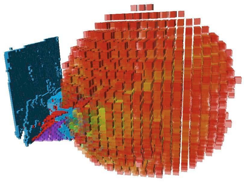
models of objects, the art gallery problem, robot exploration,              Let X be the space of 6d poses, i.e., X ∼   = R3 × SO(3) [13]
and pursuit evasion.                                                     and C ⊂ X the set of all possible configurations of the
   Traditional next best view (NBV) algorithms compute a                 sensor with respect to the kinematic motion constraints of
sequence of viewpoints until an entire scene or the surface of           the robot platform. In general, C depends on the degrees
an object has been observed by a sensor [4], [5]. Banta et al.           of freedoms (DOFs) of the robot platform. Without loss of
were using ray-tracing on a 3d model of objects to determine             generality we assume the existence of an inverse kinematic
the next best view locations revealing the largest amount of             function IK(q) with q ∈ X that generates the set of valid
unknown scene information [4]. The autonomous explorer by                configurations C. Furthermore, let Cf ree ⊂ C be the set of
Whaite and Ferrie chooses gazes based on a probabilistic                 collision free configurations in C, i.e., the set of configurations
model [6]. Although closely related to the problem of ex-                that can be taken by the sensor without colliding into obstacles.
ploring 3d environments, NBV algorithms are not necessarily              For computing Cf ree we assume the existence of collision
suitable for robot exploration [7]. Whereas sensors mounted on           detection function γ : C → {T RU E, F ALSE} that returns
mobile robots are constrained by lower degrees of freedom,               F ALSE if q ∈ Cf ree and T RU E otherwise. Note that for
sensors in NBV algorithms are typically assumed to move                  experiments presented in this paper a 5-DOF manipulator
freely around objects without any constraints. The calculation           mounted on a mobile robot platform has been used. Also note
of viewpoints, i.e., solving the question where to place a sensor        that the set of valid configurations can be precomputed for
at maximal visibility, is similar to the art gallery problem.            efficient access during the search using capability maps [14].
In the art gallery problem [8] the task is to find an optimal               The search space S can be of arbitrary shape, we only
placement of guards on a polygonal representation of 2d                  assume that its boundary δS is known but nothing is known
environments in that the entire space is observed by the guards.         about its structure. Similar to the well known concept of
   Nüchter et al. proposed a method for planning the next               occupancy grids in 2d, our 3d search reagin S is tessellated
scan pose of a robot for digitalizing 3d environments [9].               into equally sized cubes that are stored in a hierarchical 3d
They compute a polygon representation from 3d range scans                grid structure [3]. The size of the cubes is typically chosen
with detected lines (obstacles) and unseen lines (free space             according to the size of the target to be searched.
connecting detected lines). From this polygon potential next-               Let the detection set D(q) ⊂ S be the set of all locations
best-view locations are sampled and weighted according to                in S that are visible by a sensor with configuration q ∈
the information gain computed from the number of polygon                 Cf ree . The problem is to visit a sequence q1 , q1 , q3 , . . . of
intersections with a virtual laser scan simulated by ray tracing.        configurations until either the target has beenSfound or the
                                                                                                                                m
The next position approached by the robot is selected accord-            entire search space S has been explored, i.e., S \ i=1 D(qi ) is
ing to the location with maximal information gain and minimal            the empty set. Since our goal is to reduce the total search time,
travel distance. Their approach has been extended from a 2d              the sequence of configurations has to be as short as possible.
representation towards 2.5d elevation maps [10]. Newman et               Note that this problem is related to the next best view (NBV)
al. base their exploration on features, as for example walls,            problem [4] and the art gallery problem [8].
with the goal to target places of interest directly [11].
                                                                                 IV. F RONTIER -VOID -BASED E XPLORATION
   In pursuit-evasion the problem is to find trajectories of
the searchers (pursuers) in order to detect an evader moving                In this section the procedure for computing the next best
arbitrarily through the environment. Part of that problem is             viewpoints based on extracted frontiers and voids is described.
to determine a set of locations from which large portions                This is an iterative procedure where at each cycle of the
of the environment are visible. Besides 2d environments,                 iteration the following steps are performed: (1) to capture a
2.5d environments represented by elevation maps have been                3d point cloud from the environment (2) to register (align) the
considered [12].                                                         point cloud with previously acquired scans (3) to integrate the
                                                                         point cloud into the hierarchical octomap data structure (4) to
                 III. P ROBLEM F ORMULATION                              extract the frontier cells (see Section IV-A) (5) to extract the
                                                                         voids (see Section IV-B) (6) to determine and score next best
   In this section the exploration task is formally described. We        view locations (see Section IV-C) (7) to plan and execute a
first describe the model of the searcher and then the structure          trajectory for reaching the next best view location.
of the search space. Then we formulate the search problem
based on these two definitions.                                          A. Frontier cell computation
   We consider mobile robot platforms equipped with a 3d                    In this section we describe the process of extracting frontier
sensor. The 3d sensor generates at each cycle a set of n 3d              cells from the incrementally build octomap data structure.
points {p1 , p2 , . . . , pn } with pi = (xi , yi , zi )T representing   Similar to the occupancy grid classification in 2d frontier-
detected obstacles within the sensor’s field of view (FOV). The          based exploration, all 3d cells in the octomap are classified
state of the sensor, and thus the searcher, is uniquely deter-           into occupied, free, and unknown. Whereas occupied cells are
mined in ℜ3 by the 6d pose (x, y, z, φ, θ, ψ)T , where (x, y, z)T        regions covered with points from the point cloud and free cells
denotes the translational part (position) and (φ, θ, ψ)T the             are regions without points, unknown cells are regions that have
rotational part (orientation) of the sensor.                             never been covered by the sensor’s field of view.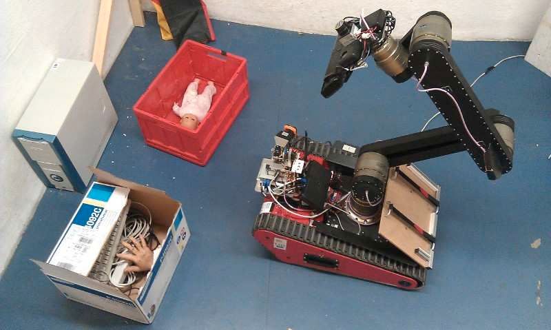
Algorithm 1 Compute N ext Best V iew
// Compute utility vectors
UV ← ∅
for all f vi = (vi , Fi , ui ) ∈ FV do
for all c ∈ corners(vi ) do
for all fi ∈ Fi do
vp ← fi
dir = normalize(pos(fi ) − c)
U V ← U V ∪ (vp, dir, ui )
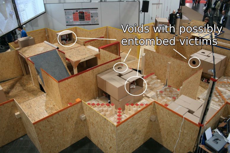
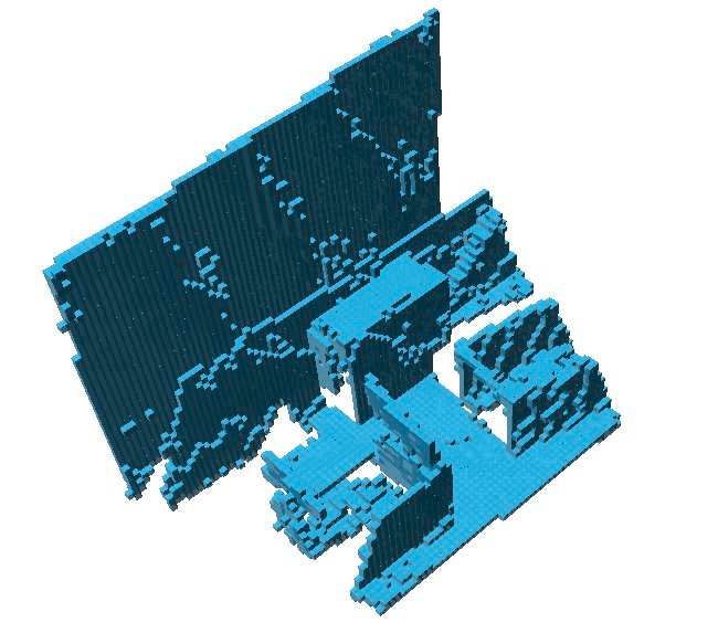
Fig. 2. This figure shows the pointcloud data integrated in an octomap end for
structure (left) and computed frontiers (red) and voids (violet). end for
end for
// Accumulate utilities in Cf ree
The set of frontier cells F consists of free cells that for all uv = (vp, dir, u) ∈ U V do
are neighboring any unknown cell. Note that occupied cells RT ← set of grid cells on the line segment of length sr
neighboring unknown cells are not belonging to F. For the in direction dir originating from vp.
sake of efficient computation, a queue storing each cell from for all c ∈ RT do
the octomap that has been updated during the last scan util (c) ← util (c) + u
integration, is maintained. By this, frontiers can be computed end for
incrementally, i.e., only modified cells and their neighbors are end for
updated at each cycle. After each update, frontier cells are
clustered by an union-find algorithm [15] forming the frontier
cluster set FC.
void cell, and λi1 , λi2 , and λi3 the eigen values of the ith
B. Void Extraction void ellipsoid.
Motivated by the work from Pauling et al. [17] voids
Similar to frontier cells, void cells are extracted from the are extracted from the set V by randomly sampling starting
octomap in a sequential manner, i.e., only cells modified by locations that are then successively expanded by a region
an incoming 3d scan are updated during each cycle. The set of growing approach until the score in Equation 2 surpasses a
void cells V contains all unknown cells that are located within certain threshold value. The procedure terminates after all void
the convex hull of the accumulated point cloud represented cells have been assigned to a cluster. The set of void clusters is
by the octomap. Extracted frontiers and voids can be seen in denoted by VC, where each cluster vi ∈ VC is described by the
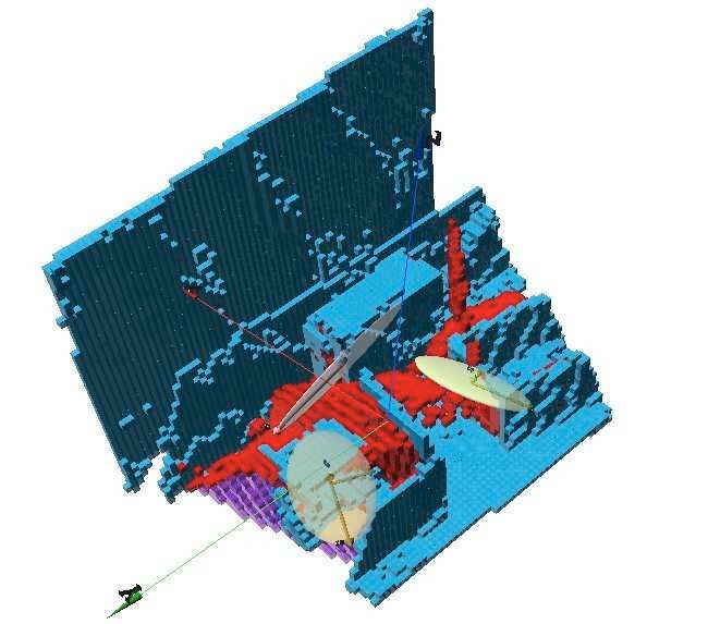
Figure 2. The convex hull of each sensor update is efficiently tuple vi = (µi , ei1 , ei2 , ei3 ,λi1 , λi2 , λi3 ), see also Figure 3.
computed by using the QHull library [16].
We are utilizing ellipsoids to build clusters of void cells
since they naturally model cylindrical, and spheroidal distri-
butions. The symmetric positive definite covariance matrix for
a set of n 3d points {p1 , p2 , . . . , pn } with pi = (xi , yi , zi )T
is given by:
1X
n
Σ= (pi − µ)T (pi − µ), (1)
n i=1
where µ P denotes the centroid of the point cloud given by
n
µ = 1/n i=1 pi . Matrix Σ can be decomposed into principle Fig. 3. On the left frontier and void cells are shown. The right side shows
the result of the clustering the void cells as three ellipsoids.
components given by the ordered eigen values λ1 , λ2 , λ3 , with
λ1 > λ2 > λ3 , and corresponding eigen vectors e1 , e2 , e3 .
The goal is to maximize the fitting between the ellipsoids and The set of void clusters VC and the set of frontier cells F
their corresponding void cells. The quality of such a fitting are combined in the final set of frontier-voids FV, where each
can be computed by the ratio between the volume of the point frontier-void f v ∈ FV is defined by the tuple f vi = (vi ∈
cloud covered by the void and the volume of the ellipsoid V, Fi ⊂ FC, ui ∈ ℜ+ ), where ui describes a positive utility
representing the void: value. In FV frontier clusters are associated with a void if they
neighbor the void cluster. Utility ui is computed according to
Ni R 3 the expectation of the void volume that will be discovered,
Si = 4 , (2)
3 πλi1 λi2 λi3
which is simply the volume of the void.
where Ni denotes the number of void cells inside the ellipsoid,
C. Next Best View Computation
R the resolution of the point cloud, i.e., the edge length of a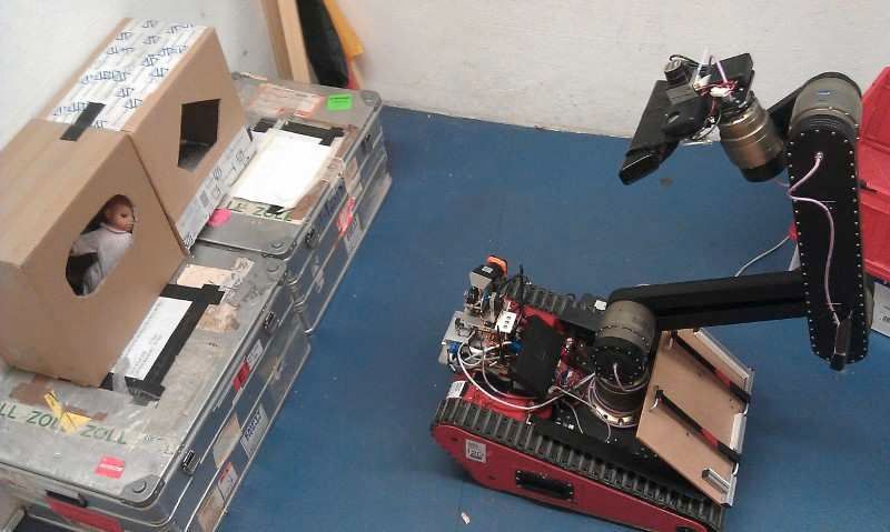
View # Integration time (s) Search Time (s) Void Utility
The computation of the next best view has the goal to Cells (dm3 )
identify the configuration of the sensor from which the max- 1 3.07 22.91 1245 19.45
imal amount of void space can be observed. As shown by 2 3.21 30.27 988 15.44
3 3.12 99.22 739 11.55
Algorithm 1 this is carried out by generating the set of utility 4 3.51 66.85 306 4.78
vectors U V by considering each frontier cell and associated 5 4.20 00.01 0 0.0
void cluster from the set of frontier-voids f vi ∈ FV. For TABLE I
each uv ∈ U V ray tracing into Cf ree is performed in order to T HIS TABLE SHOWS THE RESULTS FOR THE FIRST RUN . E ACH ROW
update the expected utility value of possible viewpoints. Ray REPRESENTS ONE SCAN INTEGRATION AND NEXT BEST VIEW
tracing is performed efficiently on the octomap and at each COMPUTATION .
visited cell of the grid the utility value from the void from
which the ray originates is accumulated. In Algorithm 1 sr
denotes the maximal sensor range, function pos(.) returns the View # Integration time (s) Search Time (s) Void Utility
Cells (dm3 )
3d position of a grid cell, and normalize(.) is the unit vector. 1 3.83 43.58 2292 35.81
corners(vi ) is a function returning the center and the set of 2 3.25 53.32 392 6.13
extremas of a void clusterSvi = (µi , ei1 , ei2 , ei3 ,λi1 , λi2 , λi3 ), 3 2.99 53.28 167 2.61
4 2.79 67.90 120 1.88
i.e. corners(vi ) = µi ∪ j∈{1,2,3} µi ± λij · eij . 5 3.87 68.53 1615 25.23
6 4.46 14.49 103 1.61
7 4.11 3.35 0 0.0
TABLE II
T HIS TABLE SHOWS THE RESULTS FOR THE SECOND RUN . E ACH ROW
REPRESENTS ONE SCAN INTEGRATION AND NEXT BEST VIEW
COMPUTATION .
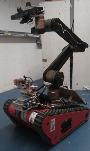
of one meter. It is shown in the top left image in Figures 5
and 6. During the experiments the base was stationary while
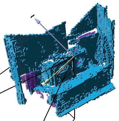
Fig. 4. The left image shows the computed utility vectors. On the right
the accumulated utilities pruned by the workspace are shown from red (low), the manipulator was used for the search. For 3d obvervations
yellow (medium) to green (high). we use a Microsoft Kinect RGBD-camera on the sensorhead.
The space of view points is then pruned by intersecting B. Results
it with the sensor’s workspace, i.e., locations that are not
We conducted experiments in two different settings. The
reachable by the sensor due to the kinematic motion model
first setting displayed in Figure 5 has a computer and two
of the robot or due to obstacles in the way, are removed. This
boxes that are open on the top as well as some two-by-fours.
can efficiently be implemented by using capability maps [14].
The second setting shown in Figure 6 features two larger
An example is given in Figure 4.
closed boxes and smaller boxes with small openings.
In the last step of the procedure the generated set of
For both experiments the robot was positioned in an initial
viewpoints is taken as a starting point for determining the next
start position. Each execution of one view consists of: Inte-
best view configuration of the sensor. For this purpose valid
grating the scan into the world representation, computing the
camera orientations (φ, θ, ψ) are sampled at the viewpoints
next best view configuration, and moving the sensor to the
c sorted by util(c) for computing the set of valid sensor
next best view position configuration. Views were executed
configurations Csens ⊂ Cf ree . Each ci ∈ Csens is defined
until the algorithm reports that there are no more void cells
by the tuple (xi , yi , zi , φi , θi , ψi , Ui ), where xi , yi , zi denote
that are reachable by the manipulator, i.e. the algorithm returns
the viewpoint location, (φi , θi , ψi ) a valid orientation at this
a utility of 0 for the best view.
viewpoint, and Ui denotes the expected observation utility
The results of both experiments are shown in Table I and
for the configuration computed by raytracing the sensors field
Table II. The integration time notes the time to integrate the
of view from the pose (xi , yi , zi , φi , θi , ψi ). The computation
scan into the octree and compute the frontier and void property
stops after N valid poses have been computed in Csens . In our
incrementally. Search time gives the time to search for the
experiments we used N = 50. Finally, the next best sensor
next best view. The last two columns list the expected number
configuration is determined by:
of void cells to be seen by the view and the corresponding
c∗ = arg max Ui . (3) volume.
ci ∈Csens
V. E XPERIMENTAL R ESULTS VI. C ONCLUSIONS
A. Experimental Platform We introduced a novel approach for solving the problem of
The robot is a Mesa Robotics matilda with a Schunk selecting next best view configurations for a 3d sensor carried
custom-built 5-DOF manipulator that has a work space radius by a mobile robot platform that is searching for objects in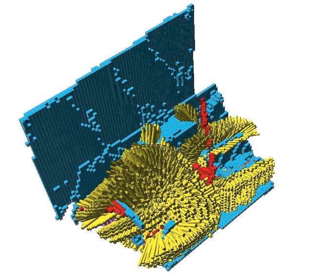
Fig. 5. The figure shows the first experiment. In the top left the experiment setting is displayed. The consecutive images show the best views chosen by the
algorithm from the current world representation. The bottom left image shows the final result.

Fig. 6. The figure shows the second experiment. In the top left the experiment setting is displayed. The consecutive images show the best views chosen by
the algorithm from the current world representation. The bottom left image shows the final result.

unknown 3d space. Our approach extends the well known 2d                       be improved in order to be applicable in real-time. Future
frontier-based exploration method towards 3d environments by                   improvements will deal with a more compact representation
introducing the concept of voids.                                              of the inverse kinematics of the robot, as well as a further
   Although the number of sensor configurations in 3d is sig-                  exploitation of the hierarchical structure for accelerating the
nificantly higher than in 2d, experimental results have shown                  search procedure.
that frontier-void-based exploration is capable to accomplish                     We also plan to evaluate the approach on different robot
an exploration task within a moderate amount of time. Due                      platforms, such as unmanned aerial vehicles (UAVs) and
to the computation of utility vectors from void-frontier com-                  snake-like robots, as well as extending the empirical evaluation
binations the search space of viewpoint configurations of the                  for various types of environments, such as represented by
sensor was drastically reduced. As a comparison perspective                    realistic point cloud data sets recorded at USAR training sites.
consider that the robot’s workspace discretized to 2.5cm
contains 444 925 nodes. A rough angular resolution of 10
degrees will result in 444 925·363 ≈ 2.08·1010 configurations.                                         ACKNOWLEDGMENTS
   The hierarchical octomap structure allowed us to perform
efficient ray tracing and neighbor query operations, which are                   This work was supported by Deutsche Forschungsgemein-
typically expensive when working with 3d data.                                 schaft in the Transregional Collaborative Research Center
   However, the performance of our approach needs still to                     SFB/TR8 Spatial Cognition project R7-[PlanSpace].
R EFERENCES                                        [9] A. Nüchter, H. Surmann, and J. Hertzberg, “Planning robot motion for
                                                                                   3d digitalization of indoor environments,” in Proceedings of the 11th
[1] A. Jacoff, B. Weiss, and E. Messina, “Evolution of a performance               International Conference on Advanced Robotics (ICAR ’03), 2003, pp.
    metric for urban search and rescue robots,” in Performance Metrics for         222–227.
    Intelligent Systems, 2003.                                                [10] D. Joho, C. Stachniss, P. Pfaff, and W. Burgard, “Autonomous Explo-
[2] B. Yamauchi, “A frontier-based approach for autonomous exploration,”           ration for 3D Map Learning,” Autonome Mobile Systeme 2007, pp. 22–
    in Proceedings of the IEEE International Symposium on Computational            28, 2007.
    Intelligence in Robotics and Automation, Monterey, CA, 1997, pp. 146–     [11] P. Newman, M. Bosse, and J. Leonard, “Autonomous feature-based
    151.                                                                           exploration,” in IEEE International Conference on Robotics and Au-
[3] K. M. Wurm, A. Hornung, M. Bennewitz, C. Stachniss, and                        tomation (ICRA), 2003.
    W. Burgard, “OctoMap: A probabilistic, flexible, and compact 3D           [12] A. Kolling, A. Kleiner, M. Lewis, and K. Sycara, “Pursuit-evasion
    map representation for robotic systems,” in Proc. of the ICRA 2010             in 2.5d based on team-visibility,” in Proceedings of the IEEE/RSJ
    Workshop on Best Practice in 3D Perception and Modeling for Mobile             International Conference on Intelligent Robots and Systems, 2010, pp.
    Manipulation, Anchorage, AK, USA, May 2010. [Online]. Available:               4610–4616.
    http://octomap.sf.net/                                                    [13] S. M. LaValle, Planning Algorithms. Cambridge, U.K.: Cambridge
[4] J. Banta, Y. Zhieng, X. Wang, G. Zhang, M. Smith, and M. Abidi, “A             University Press, 2006, available at http://planning.cs.uiuc.edu/.
    ”Best-Next-View“ Algorithm for Three-Dimensional Scene Reconstruc-        [14] F. Zacharias, C. Borst, and G. Hirzinger, “Capturing robot workspace
    tion Using Range Images,” Proc. SPIE (Intelligent Robots and Computer          structure: representing robot capabilities,” in Proceedings of the IEEE
    Vision XIV: Algorithms), vol. 2588, 1995.                                      International Conference on Intelligent Robots and Systems (IROS2007),
[5] H. Gonzalez-Banos and J. Latombe, “Navigation strategies for exploring         2007, pp. 4490–4495.
    indoor environments,” The International Journal of Robotics Research,     [15] R. E. Tarjan and J. van Leeuwen, “Worst-case analysis of set union
    vol. 21, no. 10-11, p. 829, 2002.                                              algorithms,” Journal of the ACM, vol. 31, no. 2, pp. 245–281, 1984.
[6] P. Whaite and F. Ferrie, “Autonomous exploration: Driven by uncer-        [16] C. B. Barber, D. P. Dobkin, and H. Huhdanpaa, “The quickhull algo-
    tainty,” IEEE Trans. PAMI, vol. 19, no. 3, pp. 193–205, 1997.                  rithm for convex hulls,” ACM TRANSACTIONS ON MATHEMATICAL
[7] H. Gonzalez-Banos, E. Mao, J. Latombe, T. Murali, and A. Efrat,                SOFTWARE, vol. 22, no. 4, pp. 469–483, 1996.
    “Planning robot motion strategies for efficient model construction,” in   [17] F. Pauling, M. Bosse, and R. Zlot, “Automatic segmentation of 3d laser
    Proc. of the 9th International Symposium on Robotics Research (ISRR).          point clouds by ellipsoidal region growing,” in Australasian Conference
    Springer, Berlin, 2000, pp. 345–352.                                           on Robotics and Automation, 2009.
[8] T. Shermer, “Recent results in art galleries,” Proceedings of the IEEE,
    vol. 80, no. 9, pp. 1384–1399, 1992.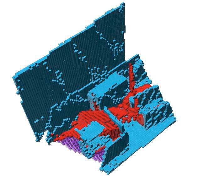
You can also read