A Multi-Variate Triple-Regression Forecasting Algorithm for Long-Term Customized Allergy Season Prediction
←
→
Page content transcription
If your browser does not render page correctly, please read the page content below
A Multi-Variate Triple-Regression Forecasting Algorithm for
                                                          Long-Term Customized Allergy Season Prediction
                                                                                      Xiaoyu Wu1 , Zeyu Bai2 and Youzhi Liang3

                                              Abstract— In this paper, we propose a novel multi-variate            in the allergy season, and the number threshold δN which
                                           algorithm using a triple-regression methodology to predict the          is the minimum number of typical days within a week
                                           airborne-pollen allergy season that can be customized for each          (7 consecutive days) in the allergy season. The start
                                           patient in the long term. To improve the prediction accuracy, we
                                           first perform a pre-processing to integrate the historical data of      date of allergy season is defined as the day, during the
                                           pollen concentration and various inferential signals from other         following week of which the number of typical days (pollen
arXiv:2005.04557v2 [stat.AP] 31 Jul 2020

                                           covariates such as the meteorological data. We then propose             concentration > δC ) is at least δN . Both δC and δN can be
                                           a novel algorithm which encompasses three-stage regressions:            customized according to different allergy sensitivity level
                                           in Stage 1, a regression model to predict the start/end date            of individuals. For example, if δC = 120 and δN = 4, the
                                           of a airborne-pollen allergy season is trained from a feature
                                           matrix extracted from 12 time series of the covariates with             standard deviation of the start date, the end date and the
                                           a rolling window; in Stage 2, a regression model to predict             length of allergy season are 19.9 days, 41.4 days and 47.2
                                           the corresponding uncertainty is trained based on the feature           days, respectively, from the year 2003 to year 2019.
                                           matrix and the prediction result from Stage 1; in Stage 3,                 Univariate forecasting methodologies, such as Exponential
                                           a weighted linear regression model is built upon prediction             Smoothing, ARIMA and T-BATS, can achieve expected
                                           results from Stage 1 and 2. It is observed and proved that
                                           Stage 3 contributes to the improved forecasting accuracy and            performance on time series data with a strong signal of level,
                                           the reduced uncertainty of the multi-variate triple-regression          trend and seasonality [9]–[11]. In addition to the classic
                                           algorithm. Based on different allergy sensitivity level, the            univariate models, the use of network and neural network
                                           triggering concentration of the pollen         the definition of        architectures, such as convolutional neural network (CNN)
                                           the allergy season can be customized individually. In our               and recurrent neural network (RNN) furthers the scope of
                                           backtesting, a mean absolute error (MAE) of 4.7 days was
                                           achieved using the algorithm. We conclude that this algorithm           application [12, 13]. Ordinary/Partial differential equations
                                           could be applicable in both generic and long-term forecasting           used widely in the field of physics and robotics shed light on
                                           problems.                                                               the machine learning models, further driving the univariate
                                                                                                                   forecasting investigation recently [14]–[18].
                                                                  I. I NTRODUCTION                                    However, univariate forecasting methodologies exhibit
                                              Airborne-pollen allergy is prevalent, affecting up to                underperformance in the context of cyclic intermittency,
                                           40% of the total population worldwide [1, 2]. The                       in particular for predicting the start date and the end
                                           long-term customized forecasting of pollen allergy provides             date of the allergy season [19]. In the scenario of
                                           individuals with guidance for travel planning and medication            airborne-pollen allergy season prediction, the concentration
                                           planning [3]–[5]. For pharmaceutical companies, the demand              of pollen, primarily produced by plants, is closely dependent
                                           of medication for pollen allergy treatment, in addition to the          on local environmental conditions like the weather and
                                           sales and operations planning for supply chain management,              geography, necessitating the integration of the meteorological
                                           further necessities the forecasting of the start/end date of the        information into the forecasting methodology [20, 21].
                                           allergy season [6]–[8].                                                 Univariate models, such as Holt-Winters exponential
                                              In Fig. 1, the concentration of pollen across the years from         smoothing, ARIMA and Facebook Prophet model, are unable
                                           2004 to 2008 is shown. We observe a significant change                  to integrate other time-varying covariates, in particular the
                                           of the start date and end date for varying years with no                weather information such as the precipitation, temperature
                                           explicit trend. For example, the allergy seasons in 2005 and            and wind [22, 23].
                                           in 2007 exhibit almost no overlapping; the length of the                   In this paper, we propose a multi-variate triple-regression
                                           allergy season in 2004 roughly doubles that in any other                algorithm to predict the airborne-pollen allergy season
                                           year.                                                                   in the long term, i.e. the start date and end date of
                                              For a more rigorous definition of the allergy season                 the season. The triggering concentration of the pollen
                                           tailored for each patient, we introduce the concentration               the definition of the allergy season can be customized
                                           threshold δC which is the minimum customized                            as aforementioned. The proposed algorithm leverages the
                                           concentration requirement of pollen for a typical day                   inferential signal from other covariates to make long-term
                                                                                                                   accurate predictions, and uses a novel three-stage modelling
                                             1 Boston University, Boston MA 02215, Email: xywu@bu.edu              approach to improve forecasting performance. In particular,
                                             2 University
                                                        of California Los Angeles, Los Angeles, CA 90095, Email:   we take into consideration the other 11 covariates including
                                           zeyubai21@engineering.ucla.edu
                                             3 Massachusetts Institute of Technology, Cambridge MA 02139, Email:   the history of temperature, wind and precipitation in addition
                                           youzhil@mit.edu                                                         to the historical data of pollen concentrations. The prediction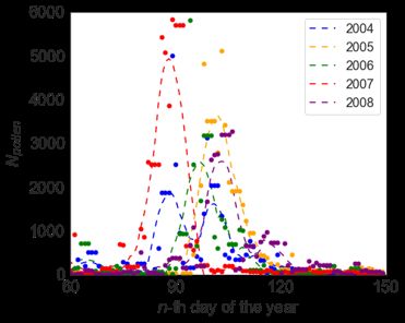
results from early stage(s) are used in later regressions to the three-stage regression can guarantee its uncertainty to be
further improve the accuracy and reduce the uncertainty of smaller than that using only one-stage regression. The proof
prediction. is given for a simplified problem as follows.
Fig. 1: The concentration of pollen as a function of the n-th day of
the year within a 120-day range, i.e. the count of pollen in a cubic
meter of air, measured per day for the year from 2004 to 2008.
The dashed lines indicate smoothed trend using the SavitzkyGolay
filter, merely serving for the visualization.
II. A LGORITHM
The proposed algorithm encompasses a three-stage Fig. 2: Data pipeline of the proposed triple-regression algorithm
regression for the start/end date of the allergy season with a nomenclature. The feature matrix from pre-processing is the
input for Stage 1; the outcome from pre-processing and Stage 1 is
prediction, together with a pre-processing for the feature the input for Stage 2; the regression results from Stage 1 and Stage
extraction. The data pipeline and the regression algorithm 2 are used in Stage 3.
are outlined in Fig. 2. In the pre-processing, a total of Nf
(=30) time series selected features are extracted by applying
We may assume that each prediction in the first-stage
a 14-day rolling window to each of the n (=12) original time
regression ŷi follows a Gaussian distribution:
series vectors xi , including the pollen concentration history,
temperature history, wind history, participation history, etc. ŷi ∈ N (µi , σi2 ), (1)
The feature matrix corresponding to xi is denoted as
(i) (1:n)
XN ×Nf , and the ensemble feature matrix is XN ×Nf ×n . The where the variance σi is assumed to be constant σ0 , and
ensemble feature matrix is then fed into the three-stage µi is theoretically constrained by a linear relationship given
regression. In Stage 1, a Gradient Boosting model to predict the predictions are made at consecutive days zi . To set
the start/end date is trained on a training set S1 which up the problem of a multi-linear regression in general,
(1:n)
is based on the feature matrix XN ×Nf ×n . The ground we may consider p independent variables x1 , ..., xn and
truth for the start/end date of allergy season is determined one dependent variable y. Suppose we have n (n > p)
following the definition after we select appropriate pollen observations,
concentration threshold δC and number threshold δN . The X
(1:n)
vector of prediction is given by ŷ = fy (XN ×Nf ×n )|S1 . ŷi = β0 + βi zij + i , i = 1, ..., n, (2)
In Stage 2, we select another training set S2 based on the
(1:n) where βi are the coefficients of the i-th dependent variable
feature matrix XN ×Nf ×n and the predicted start/end date
xi . Our goal is to minimize the sum of the weighted squared
ŷ from Stage 1 to train another Gradient Boosting model
residuals (errors) i . Thus, the cost function is:
to predict the uncertainty in ŷ. The vector of uncertainty
(1:n) 2
is given by û = fu (ŷ, XN ×Nf ×n ))|S2 . In Stage 3, we n n
p
perform a weighted linear regression on ŷ based on the
X X X
wi 2i = wi ŷi − β0 − βj zij , (3)
linear constraint on start/end date predictions at consecutive i=1 i=1 j=1
days ahead of the allergy season. The weights are assigned
according to the predicted uncertainty û. Thus, the final where the weights wi is provided by the inverse of the
predicted start/end date of the allergy season is obtained by uncertainty û2i |(2) from the regression results in Stage 2,
ŷ ∗ = fW L (ŷ)|W = û. wi = 1/σi2 |(2) = 1/û2i |(2) . No analytical solution can
Although one can opt to terminate the algorithm at Stage be obtained for a set of random weights. Without loss
1 when the predictions are already made, we emphasize that of generality, we can focus on a simplified scenario with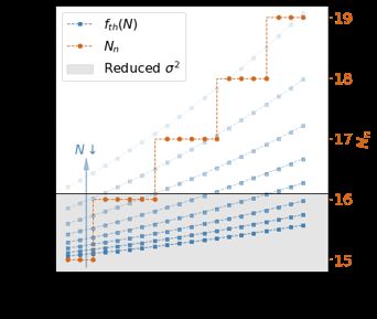
uniform weights, and the linear regression results can be
expressed as:
Cov(Z, Y )
Ŷ = E[Y ] + (Z − E[Z]), (4)
Var(Z)
where E[Y ] is the expectation of random variable Y ,
Cov(Z, Y ) is the covariance of random variable Z and Y ,
and Var(Z) is the variance of random variable Z.
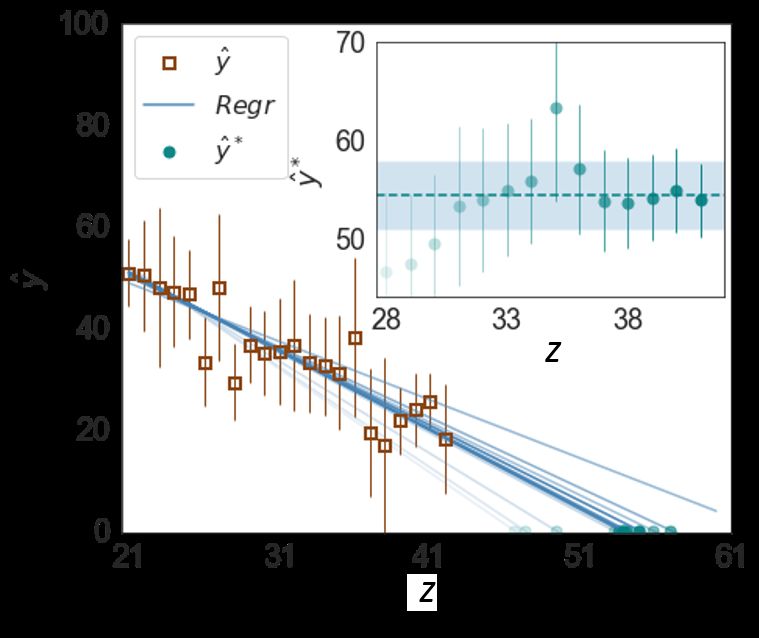
Fig. 4: Start date ŷ predicted in Stage 1, as a function of the z-th
day of the year 2005, where the error bar indicates the standard
deviation predicted in Stage 2. Straight lines are the weighted linear
regression results with different number of predictions considered.
(Inset) Final prediction of the start date ŷ ∗ predicted in Stage 3, as
a function of the z-th day of the year. Shaded area indicates the
band of standard deviation.
Thus, the standard deviation of ŷ ∗ is approximated by
s
Fig. 3: Threshold function fth (N ), and minimum number of σ 02 (β̂0 ) σ 02 (β̂1 )
days Nn to reduce uncertainty, as functions of the regression σ(ŷ ∗ ) = ŷ ∗ +
coefficient β0 with varying number of days N used for prediction. β̂02 β̂12
The shaded area indicates the regime where the variance using
s
β̂0 σ 02 1 x2 σ 02
a three-stage regression is reduced compared with the one-stage
1
=− +P 2
+ P 2
regression counterpart. Note that β1 is assumed to be 1 under the β̂1 β̂0 2 n (x i − x) β̂12 (xi − x)
condition of ideal scenario. (8)
Utilizing the third-stage regression, we aim for a reduced
In the context of predicting the start/end date of the allergy
variance, i.e. σ 2 (ŷ ∗ ) < σ02 . In other words, the uncertainty
season, the only independent variable in the weighted linear
should be reduced from the one-stage regression result. It
regression is the date zi at which the prediction is made.
is obvious that a minimum number of days Nn where the
Thus, we only have two non-zero coefficients, β0 and β1 , to
predictions are made in Stage 1 is required to guarantee the
be learned from the regression. The variance of the predicted
reduced uncertainty. We can calculate Nn by first defining
coefficient can be approximated by [24]:
the threshold function:
1 z2
σ 2 (β̂0 ) = σ 02
+
n P N
,
1 1 x2 β̂02 /β̂12
(zi − z)2 fth (Nn ) = + + ,
0 (5) Nn β̂12 Nn N
Pn N
Pn
1 (xi − x)2 (xi − x)2
σ 2 (β̂1 ) = σ 02 N
, 0 0
P (9)
(zi − z)2
0
then setting fth (Nn ) to 1, indicating that the uncertainty does
02 not change after the weighted linear regression.
It can be shown that σ is related to the uncertainty from
the Gradient Boosting regression in Stage 1 through the
III. R ESULTS AND D ISCUSSION
following formula:
σ2 To guarantee a reduced uncertainty in the three-stage
σ 02 = 0 . (6) regression compared with the one-stage regression, we
N
obtain the minimum number of days, Nn , used for making
The final prediction of the start/date date ŷ ∗ is given by the
predictions. In Fig. 3, we plot the threshold function fth (N )
z-intercept of the line from the weighted linear regression:
as a function of the coefficient β0 with varying N . The
β0 shaded area in Fig. 3 indicates the regime where the
ŷ ∗ = − (7) three-stage regression has a reduced uncertainty.
β1Therefore, the corresponding minimum number of days “Allergenic pollen and pollen allergy in europe,” Allergy, vol. 62, no. 9,
Nn for a specific β0 value can be obtained from the threshold pp. 976–990, 2007.
[2] J. Sánchez-Mesa, C. Galán, J. Martı́nez-Heras, and
function which satisfies fth (N ) < 1 and has the smallest C. Hervás-Martı́nez, “The use of a neural network to forecast
N among all threshold functions. As β0 increases, the daily grass pollen concentration in a mediterranean region: the
value of threshold function increases, reflecting an increased southern part of the iberian peninsula,” Clinical & Experimental
Allergy, vol. 32, no. 11, pp. 1606–1612, 2002.
minimum number of days Nn is required. [3] M. Prank, D. S. Chapman, J. M. Bullock, J. Belmonte, U. Berger,
We apply the data pipeline and three-stage regression A. Dahl, S. Jäger, I. Kovtunenko, D. Magyar, S. Niemelä, et al.,
algorithm to the dataset described in Section II to predict the “An operational model for forecasting ragweed pollen release and
dispersion in europe,” Agricultural and forest meteorology, vol. 182,
start date of the allergy season. The ground truth of the start pp. 43–53, 2013.
date of the allergy season is set by the thresholds, δC = 120 [4] C. Arizmendi, J. Sanchez, N. Ramos, and G. Ramos, “Time
and δN = 4, i.e., for seven consecutive days after the start series predictions with neural nets: application to airborne pollen
forecasting,” International journal of biometeorology, vol. 37, no. 3,
day, the number of days when the pollen concentrations is pp. 139–144, 1993.
greater than δC is at least δN . [5] A. Ranzi, P. Lauriola, V. Marletto, and F. Zinoni, “Forecasting airborne
In Fig. 4, we show the mean ŷ predicted in Stage 1, pollen concentrations: Development of local models,” Aerobiologia,
vol. 19, no. 1, pp. 39–45, 2003.
and the corresponding error bar, which is the standard [6] N. Singh, S. J. Olasky, K. S. Cluff, and W. F. Welch Jr, “Supply chain
deviation σ(ŷ) predicted in Stage 2 as functions of the demand forecasting and planning,” July 18 2006. US Patent 7,080,026.
z-th day of the year 2005. The models to predict ŷ and [7] S. Jaipuria and S. Mahapatra, “An improved demand forecasting
method to reduce bullwhip effect in supply chains,” Expert Systems
σ(ŷ) are trained using the dataset from year 2003 and with Applications, vol. 41, no. 5, pp. 2395–2408, 2014.
2004 respectively. The blue lines in decreasing transparency [8] Y. Barlas and B. Gunduz, “Demand forecasting and sharing strategies
represent weighed linear regression results with increasing to reduce fluctuations and the bullwhip effect in supply chains,”
Journal of the Operational Research Society, vol. 62, no. 3,
number of predictions ŷ used, where the inverse of the pp. 458–473, 2011.
uncertainty σ(ŷ) serves as the weights. The green circles [9] E. S. Gardner Jr, “Exponential smoothing: The state of the art,” Journal
locates at the z-intercept represents the final prediction made of forecasting, vol. 4, no. 1, pp. 1–28, 1985.
[10] S. C. Hillmer and G. C. Tiao, “An arima-model-based approach to
in Stage 3. It is manifested in the Fig. 4 (Inset) that the seasonal adjustment,” Journal of the American Statistical Association,
prediction converges to Day 54 as the number of days vol. 77, no. 377, pp. 63–70, 1982.
accounted increases, while the actual start date is Day 51 [11] H. Hassani, E. S. Silva, N. Antonakakis, G. Filis, and R. Gupta,
“Forecasting accuracy evaluation of tourist arrivals,” Annals of Tourism
for year 2005. We also performed backtesting for year 2006, Research, vol. 63, pp. 112–127, 2017.
2007 and 2008, and a mean absolute error of 4.7 days was [12] Z. Bai, R. Yang, and Y. Liang, “Mental task classification using
achieved using the triple-regression algorithm. electroencephalogram signal,” arXiv preprint arXiv:1910.03023, 2019.
[13] A. Chavez, D. Koutentakis, Y. Liang, S. Tripathy, and J. Yun, “Identify
The intercept of y-axis, coefficient β0 , indicates the statistical similarities and differences between the deadliest cancer
approximate prediction of the start/end date. types through gene expression,” arXiv preprint arXiv:1903.07847,
2019.
IV. C ONCLUSIONS [14] Y. Chen, B. Yang, Q. Meng, Y. Zhao, and A. Abraham, “Time-series
forecasting using a system of ordinary differential equations,”
The airborne-pollen allergy season exhibits significant Information Sciences, vol. 181, no. 1, pp. 106–114, 2011.
[15] B. N. Oreshkin, D. Carpov, N. Chapados, and Y. Bengio, “N-beats:
variations in terms of the start/end date and the length Neural basis expansion analysis for interpretable time series
of the allergy season. Univariate models fail to extract its forecasting,” arXiv preprint arXiv:1905.10437, 2019.
seasonality or trend and fail to integrate other covariates such [16] Y. Liang, A. E. Hosoi, M. F. Demers, K. D. Iagnemma, J. R.
Alvarado, R. A. Zane, and M. Evzelman, “Solid state pump using
as the temperature and precipitation. electro-rheological fluid,” June 4 2019. US Patent 10,309,386.
In our proposed triple-regression algorithm, (a) the pollen [17] R. Fish, Y. Liang, K. Saleeby, J. Spirnak, M. Sun, and X. Zhang,
allergy season can be customized based on each individual’s “Dynamic characterization of arrows through stochastic perturbation,”
arXiv preprint arXiv:1909.08186, 2019.
allergy sensitivity level, (b) the predictions are obtained [18] Y. Liang, J. R. Alvarado, K. D. Iagnemma, and A. Hosoi, “Dynamic
based on the historical data of pollen concentration together sealing using magnetorheological fluids,” Physical Review Applied,
with other 11 covariates, (c) most importantly, the uncertainty vol. 10, no. 6, p. 064049, 2018.
[19] J. H. Stock and M. W. Watson, “A comparison of linear and nonlinear
of the prediction in Stage 3 can be reduced given that the univariate models for forecasting macroeconomic time series,” tech.
minimum number of predictions obtained from Stage 1 is rep., National Bureau of Economic Research, 1998.
satisfied. The final prediction in Stage 3 converges to a mean [20] K. K. R. Samal, K. S. Babu, S. K. Das, and A. Acharaya, “Time
series based air pollution forecasting using sarima and prophet model,”
value with the increasing number of predictions obtained in Proceedings of the 2019 International Conference on Information
from Stage 1. The weighted linear regression further improve Technology and Computer Communications, pp. 80–85, 2019.
the accuracy by integrating the uncertainty predicted in Stage [21] R. Meese and J. Geweke, “A comparison of autoregressive univariate
forecasting procedures for macroeconomic time series,” Journal of
2. In our backtesting, a mean absolute error of 4.7 days was Business & Economic Statistics, vol. 2, no. 3, pp. 191–200, 1984.
achieved using the triple-regression forecasting algorithm. [22] R. Fildes and E. J. Lusk, “The choice of a forecasting model,” Omega,
We conclude that this algorithm could be useful in both vol. 12, no. 5, pp. 427–435, 1984.
[23] A. M. De Livera, R. J. Hyndman, and R. D. Snyder, “Forecasting time
generic and long-term forecasting problems. series with complex seasonal patterns using exponential smoothing,”
Journal of the American statistical association, vol. 106, no. 496,
R EFERENCES pp. 1513–1527, 2011.
[24] G. James, D. Witten, T. Hastie, and R. Tibshirani, An introduction to
[1] G. DAmato, L. Cecchi, S. Bonini, C. Nunes, I. Annesi-Maesano, statistical learning, vol. 112. Springer, 2013.
H. Behrendt, G. Liccardi, T. Popov, and P. Van Cauwenberge,You can also read