Early effects of the Covid-19 on the Tourism industry: Evidence from the three major cruise companies

Early effects of the Covid-19 on the Tourism
 industry: Evidence from the three major cruise
 companies
 Theodoros Daglis
 National Technical University of Athens

Abstract:

The Covid-19 pandemic has shifted investors’ preferences away from the cruise companies’
stocks as the lockdown measures totally suspended the services of these companies. In this
paper, we examine three of the biggest companies’ stocks, namely the Carnival Corporation
(CCL), the Royal Caribbean (RCL) and the Norwegian Cruise Line (NCLH) during the
Covid-19 spread and the lockdown measures. Using relevant time series specifications, we
establish a hypothesis regarding the effect of the Covid-19 pandemic on these three stocks.
Based on our findings, the three stocks were affected by the Covid-19 spread and more
precisely, the Covid-19 spread provides useful information for the predicting and forecasting
of these stocks. Our findings are robust, since the out-of-sample forecasting accuracy of the
alternative model employed, that explicitly incorporate the pandemic induced by the SARS-
COV-2 virus, is superior to the baseline model.
Keywords: COVID-19; tourism; cruise; stocks

1. Purpose
The recent Covid-19 pandemic has spread from one country to another, having its origin in
Wuhan-Hubei, China (Liu et al., 2020). The total cases globally amount to over 2 million
people, showing the cruel face of this pandemic (WHO, 2020). In an attempt to minimize the
spread of the virus, most economies and policy makers have taken extreme lockdown
measures that adversely affect the overall microeconomic, macroeconomic and financial
conditions in a global scale. Increased globalization and integration, of trade and financial
relations, among the various economies and institutions, makes clear that the global cost of
the pandemic will not be limited to the directly affected economies, since the indirect
spillover effects are of great importance, as well (Lee and McKibbin, 2004).

 1

Such cases are the Cruise companies that were affected both by the lockdown
measures, due to the suspension of their proper function and by the economic recession
followed by the Covid-19 spread. The lockdown measures had a very important and negative
effect on the hospitality and tourism (Bakar and Rosbi, 2020), with damages ranging from
billion to trillion dollars (Gössling et al., 2020), impacting many (if not all) of the touristic
places of the world (Nicola et al., 2020).
 Since international tourism is highly susceptible to external crisis events, it is very
interesting to investigate and quantify the factors that seem to have a negative effect on
tourism. Such a shock occurred in the cruise industry due to the Covid-19 spread. Fear has
spread for the case of the Cruise companies as cruise stocks decreased their value by 15%
approximately (Tenebruso, 2020). More analytically, some cruise stocks are expected to post
quarterly loss of $1.78 per share in its upcoming report, which represents a year-over-year
change of -369.7%. The revenues are expected to be $1.30 billion, down 73.1% from the
year-ago quarter (Zacks, 2020).
 In this paper, using relevant econometric techniques, we capture the impact of the
COVID-19 spread on the three biggest Cruise companies and more precisely on the Carnival
Corporation (CCL), the Royal Caribbean (RCL) and the Norwegian Cruise Line (NCLH)
stocks. The present paper contributes to the literature in the following ways: (a) It is the first,
to the best of our knowledge, that investigates the effect of the Covid-19 spread and the
lockdown measures on the three major cruise companies; (b) It is the first, to the best of our
knowledge, that accounts for the Covid-19 pandemic in a financial framework, using global
data on the spread of the pandemic; (c) it proposes an alternative approach to the examination
of the economic effect of disasters on the cruise companies, based on a financial framework;
and (d) it provides a robustness analysis of the findings based on out-of-sample forecasting
accuracy measures.
 The paper is structured as follows: Section 2 describes the methodology used, Section
3 presents the empirical results and Section 4 concludes the paper.

2. Methodology
In order to econometrically investigate (non-)causality between the Covid-19 confirmed cases
and the Cruise companies’ stocks, we will make use of Granger (non-)causality tests and the
state of the art step-by-step (non-) causality test, introduced by Dufour and Renault (1998)
and extended by Dufour et al. (2006).
 Additionally, in order to cross validate the fact that the Covid-19 confirmed cases are
causal and thus have predictive ability on the major Cruise companies’ stocks, we will also
make use of forecasting strategies. In detail, using a vector autoregressive model as a
baseline, we will investigate whether alternative specification that could also incorporate the
information provided by Covid-19 confirmed cases as an exogenous variable in the same
vector autoregressive model, outperforms the forecasting accuracy of the baseline model.

 2

In what follows, we offer a brief outline of the techniques and procedures used in this work.

2.1 Relevant tests
Phillips-Perron unit root test:
As a first step, we check for the potential existence of unit roots in our time series using
relevant unit root tests. More analytically, we implement the Phillips-Perron unit root test.
The null hypothesis of the test, is that the time-series contain a unit root.
Johansen co-integration test:
In case of I(1) variables, we test for cointegration among the time-series. If cointegrating
relationships are present, Error Correction Terms (ECM) have to be included in the model. In
this work, we implement the Johansen (1988) test. The trace test, tests the null hypothesis of
 < cointegrating vectors, while the maximum eigenvalue test, similarly, tests the null
hypothesis of < + 1 cointegrating vectors and the critical values are found in Johansen
and Juselius (1990).

2.2 Causality testing between Covid-19 spread and Cruise companies’ stocks
As a next step, we investigate (non-)causality between the Covid-19 confirmed cases and
the Cruise companies’ stocks, using the Granger (non-)causality tests.
Granger Non-causality
After examining the stationarity and cointegration properties of the data series, we use (non-
)Granger causality to test the predictive ability of the variables that enter the model. More
precisely, the hypothesis tested for Granger (non-)causality test is that the times series are not
Granger causal, i.e. the logarithmic Covid-19 confirmed cases do not have predictive ability
on the biggest cruise stocks. As Engle and Granger (1987) showed, if two variables are
cointegrated, an Error Correction Model (ECM) should be employed in the model in order to
capture the long-run relationship among the variables.
 The ECM Granger non-causality test involves fitting the model:

 = 0 + ∑ 
 =1 1 − + ∑ =0 2 − + −1 + (1)

where Δ is the first difference operator, Δyt and Δxt are stationary time series and εt is the
white noise error term with zero mean and constant variance. Also, μt-1 is the lagged value of
the error term of the cointegration regression.
 Next, in order to study the exact timing pattern of the causality relationship, we make
use of the state-of-the-art step-by-step causality introduced by Dufour and Renault (1998) and
extended by Dufour et al. (2006).
Step-by-step causality

 3

Based on recent advancement of the related literature of causality, Granger non-causality
tests fail to unveil the potential timing pattern of a causal relationship. In this context, in a
seminal paper in Econometrica, Dufour and Renault (1998) introduced the notion of step-by-
step or short-run causality based on the idea that two time series Xt and Yt could interact in a
causal scheme via a third variable Zt. More precisely, despite the fact that Xt could not cause
Yt one period ahead, it could cause Zt one period ahead i.e. Zt+1, and Zt could cause Yt two
periods ahead i.e. Yt+2. Therefore, Xt → Yt+2, even though Xt ↛ Yt+1.

 For testing the step by-step causality, consider the following VAR (p) model:

 = + ∑ =1 − + ∑ =0 − + (3)
where: Yt is an (1xm) vector of variables, a is a (1xm) vector of constant terms; Xt is a vector
of variables and ut is a (1xm) vector of error terms such that ( ) = =
 ( ) = ≠ , where I is the identity matrix. The lags in the baseline model
are selected using the Schwartz-Bayes Information criterion (SBIC).

 Following Dufour et al. (2006), the model described in (3) corresponds to horizon
h=1. In order to test for the existence of non-causality in horizon h, the algorithm follows
Konstantakis and Michaelides (2015).

2.3 Econometric models
A basic and classical econometric approach is the vector autoregressive model - VAR, or the
vector error correction model – VECM in presence of co-integration relationship among the
variables. In presence of co-integration relationship among the variables, we incorporate the
error correction term.
 Each variable in the model, has an equation explaining its evolution based on its own
lagged values, the lagged values of the other model variables, the error correction, and an
error term. A VECM model of order p, with exogenous variables is structured as follows:
 
 1, = 1 + ∑ ∑ ( , , − ) + ∑ ∑ ( , , − ) + 1, + 1, 
 2, = 2 + ∑ ∑ ( , , − ) + ∑ ∑ ( , , − ) + 2, + 2, (4.7)
 …
 
 { , = + ∑ ∑
 ( , , − + ∑ ∑ ( , , − ) + , + , }
 )

 n is the number of the dependent variables ( , ) of the model, is the fixed term, p is
the lag order of the dependent variables, , is the error term of each equation of the model,
and , is the error correction term, as before. In the case of exogenous variables, k is the
number of the independent or exogenous variables ( , ) of the model and q is the lag order of
the exogenous variables.

 4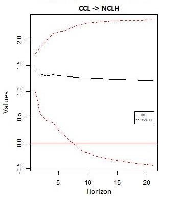

2.4 Information criterion
In this paper, we make use of the so-called Schwartz-Bayes Information criterion (SBIC)
introduced by Schwarz (1978), because it is an optimal selection criterion when used in finite
samples (Breiman and Freedman, 1983; Speed and Yu, 1992). The SBIC is derived:
 ln( ( )) ln( )
 ̂ = ≤ {−2 + }
 
where LL(k) is the log-likelihood function of a VAR(k) model, n is the number of
observations and k is the number of lags and ̂ is the optimum lag length selected.

2.5 Forecasting accuracy
In the present paper, we make use of the forecasting accuracy measures: mean absolute error
(MAE), the mean absolute percentage error (MAPE) and root mean square forecast error
(RMSFE). In general, the smaller the values of each forecasting criterion, the better the
forecasting value.
MAE
A model’s MAE for forecast horizon H is given by the following:
 1
 = ∑ 
 =0| − | (4.17)

where: ℎ is the forecast horizon of the model, are the out-of-sample forecasted values of
the model, and are the actual values. However, one of the main disadvantages of the MAE
is the fact that is has no standard scale and it is not as comparable as a percentage. To
overcome this problem we will also base our analysis on MAPE.
MAPE
A model’s MAPE is given by the expression:
 ℎ
 100 | − |
 = ∑
 ℎ | |
 =0

RMFSE
The RMSFE is used to measure the forecasting error distribution. It is given by the
expression:
 2
 = √ [( +1 − ̂ +1| ) ] (4.19)
2.6 Forecast accuracy comparison
In order to compare the forecasting accuracy of the baseline and alternative models, we use
the Diebold - Mariano test. This test was established by Diebold and Mariano (1991), for the
comparison of two forecast results.

 5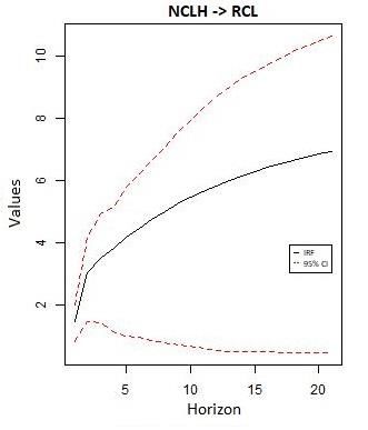

First, we define the actual values: { , = 1, … , } and two forecast values: { ̂1 , =
1, … , } and { ̂2 , = 1, … , }.

 Next, we define the forecast errors as:
 = ̂ − , = 1,2 (2.29)
 And,
 ( ) = exp{ } − 1 − (2.30)
 Function g is a loss function and l is a positive constant.

 The loss differential between the two forecasts is:
 = ( 1 ) − ( 2 ) (2.31)

 The null hypothesis of the Diebold – Mariano test is the following:
 0 : ( ) = 0
 And the respective alternative hypothesis:
 0 : ( ) ≠ 0
3. Result Analysis

3.1Data and variables
The data used in the present paper are the global Confirmed cases of the Covid-19 in daily
format and were downloaded by the John Hopkins University database and span the period
22 January 2020 until 22 May 2020. Moreover, in the present paper we used financial stocks
of the three biggest Cruise companies, namely the the Carnival Corporation (CCL), the Royal
Caribbean (RCL) and the Norwegian Cruise Line (NCLH) as derived from finance.yahoo,
and span also the period 22 January 2020 until 22 May 2020. The confirmed cases were
transformed into logarithmic scale. The descriptive statistics of the timeseries are depicted in
Table 1. Furthermore, the plots of the logarithmic confirmed Covid-19 cases and the three
CCL stock index are depicted on Figures 1-3.

Table 1: Descriptive statistics of the timeseries.

 Variable Mean Standard Deviation Min Max
 Log Confirmed Covid-19 cases 12.67 2.31 6.32 15.47
 CCL 23.46 13.72 7.97 49.30
 NCLH 25.35 18.38 7.77 58.22
 RCL 61.41 35.30 22.33 128.32

 6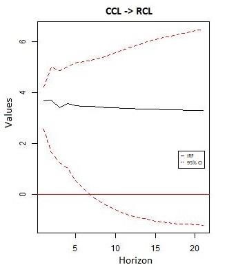

Figures 1-3: Log Confirmed Covid-19 cases and CCL, NCLH and RCL stock index,
respectively.

Figures 1-3 indicate that the logarithmic confirmed Covid-19 cases seem to have a lagged
effect on the three stocks. This fact provide a graphical evidence about the impact of the
Covid-19 spread on the Cruise companies’ stocks, a fact that needs to be investigated
thoroughly using econometric methodology.

3.2Results
 In the present work, we make use of the granger and step-by-step causalities in order
to identify whether the Covid-19 spread causes the three major Cruise companies, as captured
by the stocks of these companies. As a next step, we test the contribution of the information
derived by the Covid-19 confirmed cases on the forecasting of the aforementioned stocks. To
do so, we make use of two econometric models in the form of vector autoregressive model
(since there is connection among the three stocks). The first model, declared as he baseline,
will be a vector autoregressive model only with endogenous variables (the three stocks) and
an alternative model being the same with the baseline, augmented with one exogenous
variable, the Covid-19 global confirmed cases. The comparison of these two models, in terms
of forecasting ability, will unveil a possible contribution of the exogenous variable on the
forecasting of the three stocks.
 A first step in every econometric modeling is the unit root test. In the present paper,
we make use of the Phillips – Perron unit root test. The results are depicted in Table 2.
Table 2: Phillips – Perron unit root test results.

 Variable PP-test P-value Order of Integration
 Log_Confirmed Covid-19 cases 0.01 I(0)
 CCL 0.96 I(1)
 NCLH 0.98 I(1)
 RCL 0.96 I(1)
 Since the results in Table 2 show that the Covid-19 has no unit root, meaning that the
timeseries is stationary, this specific timeseries cannot be cointegrated and thus, it is excluded
from the cointegration test.

 7

Table 3: Johansen Cointegration test results.

 Rank of co-integration Test 10pct 5pct 1pct
 r

Table 6: Results of the SBIC criterion for the case of the Baseline and Alternative
models.

 Order SBIC for the Baseline SBIC for the Alternative
 1 2.273 -3.409
 2 2.570 -2.779
 3 2.932 -2.137
 4 3.294 -1.439
 5 3.692 -0.826
 6 4.045 -0.540
 7 4.271 -0.036
 8 4.679 0.605
 9 5.003 0.884
 10 5.352 -3.409

 Based on Table 6, the SBIC criterion indicate the lag order 1 as the most appropriate
for both models. In this case, the order of the baseline and alternative order will be selected to
be equal to 1.
 The baseline model incorporated one lag order for each endogenous variables (CCL,
NCLH and RCL). Using out of sample forecast with fixed window, for horizon H=1,2,…,20,
we forecast for approximately two months. Then, we employ the same model incorporating
as exogenous variable the logarithmic global confirmed Covid-19 cases and test again the
forecasting ability of this alternative model. We then compare the two models in terms of
forecasting ability, based on the MAE, MAPE, RMSFE and estimate the statistical
significance of the comparison based on Diebold-Mariano test. The results are depicted in
Tables 7-9.

 9

Table 7: MAE, MAPE and RSMFE forecasting accuracy of the VEC and VECX models
 for the case of CCL

Horizon MAE_VEC MAPE_VEC RMSFE_VEC MAE_VECX MAPE_VECX RMSFE_VECX
 1 0.933 0.072 0.933 0.745 0.057 0.745
 2 1.631 0.116 1.774 1.361 0.097 1.494
 3 2.601 0.168 2.996 2.234 0.144 2.602
 4 2.890 0.185 3.203 2.417 0.155 2.698
 5 2.680 0.175 2.981 2.092 0.135 2.439
 6 2.622 0.173 2.883 1.910 0.124 2.263
 7 2.418 0.161 2.707 1.700 0.111 2.102
 8 2.250 0.151 2.560 1.598 0.106 1.991
 9 2.217 0.151 2.500 1.460 0.097 1.881
 10 2.279 0.156 2.536 1.330 0.089 1.785
 11 2.317 0.159 2.551 1.242 0.083 1.706
 12 2.313 0.160 2.529 1.238 0.084 1.669
 13 2.259 0.158 2.470 1.318 0.091 1.723
 14 2.234 0.158 2.434 1.397 0.099 1.783
 15 2.265 0.161 2.453 1.442 0.103 1.803
 16 2.434 0.172 2.679 1.370 0.098 1.748
 17 2.566 0.182 2.836 1.352 0.097 1.715
 18 2.704 0.191 3.003 1.342 0.096 1.690
 19 2.870 0.202 3.217 1.319 0.094 1.657
 20 3.031 0.213 3.418 1.313 0.094 1.637

 10

Table 8: MAE, MAPE and RSMFE forecasting accuracy of the VEC and VECX models
 for the case of NCLH.

Horizon MAE_VEC MAPE_VEC RMSFE_VEC MAE_VECX MAPE_VECX RMSFE_VECX
 1 0.737 0.064 0.737 0.510 0.045 0.510
 2 1.644 0.130 1.877 1.302 0.102 1.524
 3 3.123 0.210 3.832 2.655 0.177 3.336
 4 3.919 0.254 4.578 3.315 0.214 3.918
 5 3.940 0.261 4.472 3.190 0.210 3.706
 6 4.103 0.274 4.550 3.201 0.212 3.634
 7 3.802 0.261 4.280 2.749 0.182 3.365
 8 3.613 0.254 4.084 2.420 0.161 3.148
 9 3.607 0.259 4.029 2.234 0.150 2.978
 10 3.685 0.268 4.067 2.126 0.144 2.849
 11 3.724 0.276 4.071 1.972 0.135 2.719
 12 3.741 0.282 4.059 1.826 0.125 2.604
 13 3.730 0.287 4.026 1.763 0.123 2.518
 14 3.787 0.297 4.064 1.678 0.118 2.431
 15 3.881 0.309 4.148 1.595 0.113 2.351
 16 4.116 0.327 4.449 1.590 0.113 2.308
 17 4.329 0.344 4.705 1.558 0.111 2.253
 18 4.566 0.362 5.002 1.547 0.111 2.213
 19 4.873 0.382 5.422 1.603 0.115 2.235
 20 5.171 0.402 5.813 1.644 0.118 2.246

 11

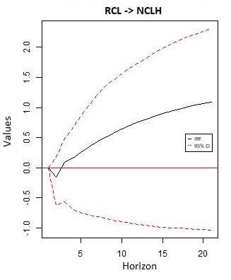
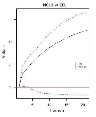
Table 9: MAE, MAPE and RSMFE forecasting accuracy of the VEC and VECX models
 for the case of RCL.

Horizon MAE_VEC MAPE_VEC RMSFE_VEC MAE_VECX MAPE_VECX RMSFE_VECX
 1 4.027 0.102 4.027 3.349 0.085 3.349
 2 5.155 0.127 5.277 4.167 0.102 4.246
 3 7.792 0.175 8.687 6.463 0.145 7.263
 4 8.872 0.196 9.658 7.180 0.159 7.832
 5 8.406 0.189 9.120 6.332 0.141 7.127
 6 8.276 0.188 8.889 5.801 0.130 6.632
 7 7.668 0.177 8.369 5.173 0.117 6.163
 8 7.151 0.167 7.927 4.884 0.112 5.853
 9 7.037 0.166 7.748 4.486 0.104 5.535
 10 7.206 0.171 7.851 4.061 0.094 5.252
 11 7.246 0.174 7.832 3.871 0.090 5.043
 12 7.201 0.175 7.745 3.887 0.092 4.968
 13 7.089 0.174 7.610 4.067 0.099 5.076
 14 7.100 0.177 7.584 4.203 0.104 5.145
 15 7.324 0.183 7.808 4.191 0.104 5.078
 16 7.969 0.197 8.753 4.044 0.100 4.938
 17 8.503 0.209 9.446 3.811 0.094 4.791
 18 8.955 0.220 9.982 3.705 0.092 4.677
 19 9.551 0.233 10.772 3.527 0.087 4.553
 20 10.128 0.246 11.511 3.365 0.083 4.438

 The results in Tables 7-9 show that the alternative model is better in terms of
 forecasting ability than the baseline, for the three stocks (CCL, NCLH, RCL). All results,
 based on the Diebold-Mariano test are statistical significant. This implies that the Covid-19
 augments the forecasting ability of the stocks of the three major cruise companies.
 Finally, using the impulse – response function, and more precisely, the orthogonalized
 impulse responses, the results indicate that the effect of the RCL on the CCL stock, is not
 statistically significant, as depicted in Figure 4 - a. In the same context, the effect of the RCL
 on the NCLH stock, is not statistically significant (Figure 4 – b). Moreover, the effect of the
 CCL on the NCLH stock, is statistically significant and positive (Figure 4 – c). This means
 that a unit shock in the CCL stocks, will lead to a positive effect in the NCLH stocks.

 12

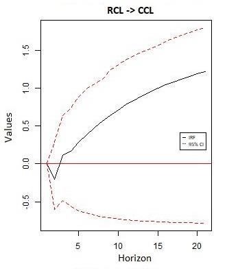
The effect of the CCL on the RCL stock, is statistically significant and positive, as depicted
in Figure 4 – d. This means that a unit shock in the CCL stocks, will lead to a positive effect
in the RCL stocks. Furthermore, the effect of the NCLH on the CCL stock, is statistically
significant and positive (Figure 4 – e). This in turn, means that a unit shock in the NCLH
stocks, will lead to a positive effect in the CCL stocks. Finally, the effect of the NCLH on the
RCL stock, is statistically significant and positive, as depicted in Figure 4 - f. This means that
a unit shock in the NCLH stocks, will lead to a positive effect in the RCL stocks.
Figure 4: Impulse response function for the endogenous variables.

 13

4. Conclusion
 In the present paper, we examine three major cruise companies’ stocks, namely the
Carnival Corporation (CCL), the Royal Caribbean (RCL) and the Norwegian Cruise Line
(NCLH) during the Covid-19 spread and lockdown measures. Using relevant time series
specifications, we establish a hypothesis regarding the effect of the Covid-19 on these three
stocks. The hypothesis is proved, as, based on our findings, the Covid-19 spread, Granger
causes and also step-by-step causes the CCL, NCLH and RCL stocks. These results indicate
that the Covid-19 spread provide useful information for the modeling of these stocks as it
affects them, econometrically speaking.
 Furthermore, the Covid-19 spread provides useful information for the forecasting of
these stocks, as shown by the forecasting comparison of the baseline and alternative models,
indicated by the forecasting criteria MAE, MAPE and RMSFE, with statistical significance of
the comparison, as shown by the Diebold-Mariano test. Our findings are robust, since the out-
of-sample forecasting accuracy of the alternative model employed, that explicitly incorporate
the pandemic induced by the SARS-COV-2 virus, are superior to the baseline model.
 The present paper findings show that the Covid-19 spread not only contributes with
statistically significant information in the modeling of the three major cruise companies’
stocks, but also increase the forecasting ability of these stocks in the 22/10 – 22/05 time
period of the year 2020. The results give credit to the impact of the Covid-19 spread on the
Cruise Companies, decreasing their revenues and impacting their stocks. This fact unveils the
great impact of the Covid-19 on the tourism industries worldwide.
 Finally, the effect of the CCL stock on the NCLH and the RCL stocks, is statistically
significant and positive, which means that CCL affects the other two stocks in a positive way.
The same case is for the NCLH stock, as it affects the CCL and RCL stocks with statistical
significant and positive shock. On the other hand, The effect of the RCL on the NCLH stock,
and also on the CCL stock, is not statistically significant. This means that the RCL cruise
company does not affect the other two major cruise companies with statistical significance.
 Shedding light to the case, a fact is that the cruise companies, during the lockdown
measures lost big portion (if not all) of their profits, leading them to severe economic
damage. This occurrence, made the traders to swap from these stocks to other commodities,
regarded as more stable.
 Summing up, the economic measures that decreased and during some period of time
totally suspended the Cruise companies’ function, and simultaneously the abandon of the
Cruise trades had an extremely negative impact on these companies, as depicted by the
modeling and forecasting, employed in the present paper. We anticipate our work to be a
starting point for more sophisticated models, testing for other factors that could play a
significant role in forecasting the various touristic industries. Clearly, future and more
extended research on the subject would be of great interest.

 14

References
Liu Ying, Gayle Albert A., Wilder-Smith Annelies and Rocklöv Joacim (2020), The reproductive
number of COVID-19 is higher compared to SARS coronavirus, Journal of travel medicine, 1-4.

WHO - World health organization (2020), Coronavirus disease 2019 (COVID-19), Situation Report –
51.

Lee J-W and W. McKibbin (2004), Estimating the Global Economic Costs of SARS In: S. Knobler,
A. Mahmoud, S. Lemon, A. Mack, L. Sivitz, and K. Oberholtzer (Editors), Learning from SARS:
Preparing for the next Outbreak, The National Academies Press, Washington DC (0-309-09154-3).

Bakar Abu Nashirah and Rosbi Sofian (2020), Effect of Coronavirus disease (COVID-19) to tourism
industry, International Journal of Advanced Engineering Research and Science, Vol-7, Issue-4,
dx.doi.org/10.22161/ijaers.74.23.

Breiman L.A. and Freedman D.F. (1983), How many variables should be entered in a regression
equation?, J. Am. Stat. Assoc. 78, pp. 131–136.

Gössling Stefan, Scott Daniel and Hall C. Michael (2020): Pandemics, tourism and global change: a
rapid assessment of COVID-19, Journal of Sustainable Tourism, OI:
10.1080/09669582.2020.1758708.

Nicola Maria, Alsafib Zaid, Sohrabic Catrin, Kerwand Ahmed, Al-Jabird Ahmed, Iosifidisc Christos,
Aghae Maliha and Aghaf Riaz (2020), The socio-economic implications of the coronavirus pandemic
(COVID-19): A review, International Journal of Surgery, 78, 185–193.

Zacks (2020), Zacks Equity Research 11 June 2020, Link: https://finance.yahoo.com/news/earnings-
preview-carnival-ccl-q2-163004606.html.

Tenebruso Joe (2020), Why Carnival, Royal Caribbean, and Norwegian Cruise Line Stocks Plunged
Today, TMFGuardian, 11-06-2020, Link: https://www.fool.com/investing/2020/06/11/why-carnival-
royal-caribbean-and-norwegian-cruise.aspx

Diebold X. Francis and Mariano S. Roberto (1991), Comparing predictive accuracy I: An asymptotic
test, Discussion paper 52, Federal reserve bank of Minneapolis, Institute for empirical
macroeconomics, , pp. 1-29.

Dufour J.-M. and Pelletier D. and Renault E. (2006), Short run and Long run Causality in Time series:
Inference, Journal of Econometrics, 132 (2): 337-362.

Dufour, J.-M., Renault, E. (1998), Short-run and long-run causality in time series: theory,
Econometrica, 66 (5): 1099–1125.

 15

Engle, F.R. and Granger, W.J.C. (1987), Co-integration and error correction: representation,
estimation, and testing, Econometrica 55 (2): 251–276.

Johansen Søren (1988), Statistical analysis of cointegration vectors, Journal of Economic Dynamics
and Control, Volume 12, Issues 2–3, Pages 231-254.

Johansen Soren, Juselius Katarina (1990), Maximum likelihood estimation and inference on
cointegration-with applications to the demand for money, Oxford Bulletin of Economics and
Statistics, 52(2): 169–210.

Phillips Peter C. B. and Perron Pierre (1988), Testing for a Unit Root in Time Series Regression,
Biometrika, Vol. 75, No. 2, pp. 335-346.

Konstantakis N. Konstantinos and Michaelides G. Panayotis, (2015), Step-by-Step Causality
Revisited: Theory and Evidence, Economics Bulletin, Volume 35, Issue 2, pages 871-877.

Speed T.P and Yu Bin (1992), Model selection and prediction: Normal Regression, Annals of the
Institute of Statistical Mathematics, Vol. 45, Issue 1, pp. 35-54.

Wooldridge J. M. (2013), Introductory Econometrics: A Modern Approach. 5th ed. Mason. OH:
South-Western.

 16