A Novel Solution for the General Diffusion
←
→
Page content transcription
If your browser does not render page correctly, please read the page content below
A Novel Solution for the General Diffusion
                                                                                 Luisiana Cundin
                                                                                 August 25, 2021
arXiv:2108.10450v1 [math-ph] 24 Aug 2021

                                                                                       Abstract
                                                      The Fisher–KPP equation is a reaction–diffusion equation originally proposed
                                                  by Fisher to represent allele propagation in genetic hosts or population. It was
                                                  also proposed by Kolmogorov for more general applications. A novel method for
                                                  solving nonlinear partial differential equations is applied to produce a unique, ap-
                                                  proximate solution for the Fisher–KPP equation. Analysis proves the solution is
                                                  counter–intuitive. Although still satisfying the maximum principle, time depen-
                                                  dence collapses for all time greater than zero, therefore, the solution is highly
                                                  irregular and not smooth, invalidating the traveling wave approximation so often
                                                  employed.
                                               Keywords— KPP equation or Fisher–KPP equation

                                           1 On the general diffusion. . .
                                           Diffusion is incontrovertibly one of the most fundamental physical processes describing the
                                           transport of energy, mass and other phenomena through space and time. The linear transfer of
                                           energy is certainly in the purview of Nature’s design, as evidenced all around us, everyday; but,
                                           nonlinear transfer has long been sought as an extension to rational systems where the medium re-
                                           acts to the gradient of concentration. A nonlinear diffusive process would describe some process
                                           that, in addition to gradient dependence, would be further dependent upon the medium response
                                           to the gradient of concentration, reacting in some nonlinear, chaotic fashion [1, 2]. The concept
                                           of some unusual medium response is predicated upon the idea that the medium carries some
                                           special reactive properties, like memory or retention or something of the sort that would account
                                           for some additional behavior atop ordinary flux allowed by the medium.
                                                It may be that any such nonlinear diffusive behavior could simply be captured in a modi-
                                           fied diffusion constant, rather, experimentalists may find unique diffusion constants for various
                                           media, and, never think it due to some reactive medium response [3, 4, 5]. In fact, any exotic,
                                           complex diffusivity should be focused upon the diffusion constant, per se, and not extricated to
                                           describe the medium response itself. In general, the media response is typically random in na-
                                           ture, as per Brownian motion; moreover, although randomness is often perceived nonlinear, it is
                                           rational nonetheless [6]. Whether it is physically possible for media to exhibit nonlinear reactive
                                           responses is certainly questionable, in fact, it may all together be not possible for such systems
                                           to exists; because, linear diffusion already describes the flux of energy and mass subject to the
                                           local gradient or concentration, therefore, already accounts for the actual medium response in
                                           its description of mass/energy transfer [7]. To ascribe additional ”nonlinear” attributes to media
                                           would imbue into physical materialé some ghost process or special physical phenomenon yet
                                           discovered.
                                                In many cases, for example, reaction–diffusion processes, as are certain chemical reactions,
                                           nonlinear diffusion equations are used in an attempt to capture the media’s actual response to
                                           changes in the gradient as the chemical reaction progresses in time and space, therefore, there is

                                                                                           1
some rationalé behind attempting to formulate some type of equation that mimics a very com-
plex, intricate play in reversible concentrations, as the chemical reaction progresses to home-
ostasis [8]. Nevertheless, to formulate or reduce such a complex process to one, all encom-
passing equation may or may not be suitable, adequate or advisable, for the process is truly an
interplay of many reaction chemical kinetic equations, interacting over time and space, with an
intricate dance in concentrations diminishing and evolving in time. Complex systems, generally
speaking, require a milieu of equations, each formulated specifically, to properly model each
element/species involved in the overall process [9]. In this manner, a researcher adequately ac-
counts for each kinetic species in the reaction and does not attempt to ’cut corners’ by reducing
the entire system to some modified ”nonlinear” system, which is often forced, in some manner,
into a one–dimensional system; this done in hopes it will mimic the system in question and admit
ease in solving.
There are many reasons the simple addition of some multiplicative medium response is not
advisable nor should be considered physically correct. Of the many reasons, Ostrogradsky’s
theorem concerning mechanics stands tall [10]. The theorem shows why no system with higher
order derivatives than second order are physically acceptable or seen in mechanics, furthermore,
it proves third order and higher systems are unstable in time and space, therefore, describe un-
realistic physical processes, or, in the least, doomed processes. All systems are bounded from
above by energy and by material properties (strengths); but, to say a system’s Hamiltonian is
unbounded from below envisions a system which allows a particle at rest to suddenly jump from
rest to some unbounded state of energy, moreover, a negative state of energy, which is improper,
to say the least. All energy is positive, although, in a relative system or coordinate system, neg-
ative energies are possible, even though, such formulations are sloppy, at best, but improper, at
worst.
Nonlinear equations admit special solutions, usually, involving hyperbolic trigonometric
equations, which are typically periodic functions and suffer from branch points, singularities and
other non-analytic properties. The fact poles exist within the domain of the solution should indi-
cate to the wary that the domain is not entire, therefore, the solution is hemmed in or restricted in
some way or another. A typical path for solving nonlinear equations involves the traveling wave
approximation, which assumes any deflection in the solution is small enough and smooth enough
to allow for equivalence under D’Alembert’s principle, thereby, enabling reduction of an equa-
tion of some dimension to a one–dimensional canonical equation, whose behavior is assumed
equivalent [11, 12]. Nonlinear equations, in general, are not smooth and this fact brings any
solution obtained via the traveling wave approximation under serious scrutiny, as will be seen
for the Fisher–KPP equation, shortly. The additional multiplicative medium response places
extraordinary restraints upon the system and any solution.
2 Fisher-KPP equation
Consider the general Fisher–KPP equation with real coefficients (D, b, r), where D describes the
diffusivity of the material under question, b the linear response of the medium (if applicable),
and r the nonlinear coefficient, viz.:
∂ ∂2
u(x,t) = D 2 u(x,t) − b u(x,t) + r u(x,t)2 /; {(D, b, r)|(D, b, r) ∈ ℜ} (1)
∂t ∂x
Assume a solution in the form of u(x,t) = G(x,t) ∗ f (x,t), where G(x,t) represents Green’s
function which solves the linear equation, inept, r = 0; viz.:
2
e−x /4Dt 2
G(x,t) = √ ⊂ e−(2π s) Dt e−bt = g(s,t), (2)
4π Dt
where symbol ⊂ is borrowed from Bracewell, indicating the Fourier transform of the given
function [13].
2Since Green’s function is a solution to the linear partial differential equation with linear
medium response already included, then the task at hand is to reduce the main equation to some
residual equation involving only the nonlinearity. Employing Green’s solution realizes several
cancellations immediately, cancelling several terms after applying the time derivative, where
partial derivatives distribute across convolution integrals, see Theorem 3. Moreover, one retains
the choice onto which function a derivative is acted upon, if the convolution integral involves
the same variable, to wit, the choice has been made to apply both spatial derivatives to Green’s
function, viz.:
′ ✘✘
∗ f )(x) + (G ∗ f ′ )(x) = ✭ ✭+ r (G ∗ f )2 (x),
✘ ✭
(G✘
✘ D (G
✭xx f )✭
✭∗✭ b (G
(x) −✭ ✭∗✭f ✭
) (x) (3)
where prime indicates derivative with respect to time.
Since all terms are removed except the nonlinear term and the corresponding time derivative
needed to cancel this term, the residual equation, viz.:
G ∗ f ′ = r (G ∗ f )2 (x) (4)
No immediate solution comes to mind for the above equation, so, a sequence of approxima-
tions for the convolution integral will be employed, namely,
Theorem 1 (Convolution integral theorem). The convolution integral is greater than or equal to
the product of both functions involved in the convolution integral
f ∗g ≥ fg (5)
Theorem 1 is true in general because the convolution integral sums an area either larger than
or equal to the area of both functions multiplied together. This approximation enables bypassing
the convolution integral and solving the resulting ordinary differential equation.
3 Zeroth approximation
With the aid of the approximation for a convolution integral, theorem 1, the residual nonlinear
equation can be transformed into a Bernoulli equation, which has an exact solution. Applying
the approximation once will yield interesting results and they will be investigated.
Firstly, equation (4) will be brought to bear in the frequency domain to yield a zeroth approx-
imation. In the original domain, the approximation must be applied to two convolution integrals,
whereby, in the codomain, the approximation is only for one convolution integral, therefore, the
overall approximation should be closer. In the transform domain, the residual nonlinear equation
takes on the following form, plus, the approximation, after applying theorem 1, is to the right of
the inequality, viz.:
gFt = r (gF ∗ gF) (s) ≥ gFt = rg2 F 2 (6)
The approximation initiates a set of applications to yield a solution, viz.:
gFt =rg2 F 2 ,
Ft
=rg,
F2
1
Z
− =C(s) + r g dt, finally,
F
1
F= R ,
C(s) − r g dt
where C(s) is a constant of integration.
The solution states the following, in the frequency domain, viz.:
u(s,t) = gF (7)
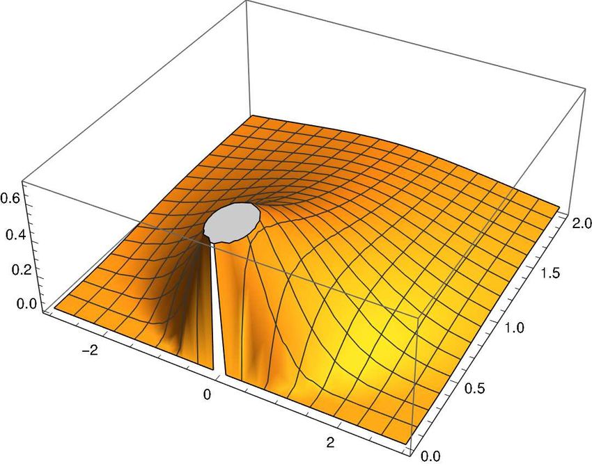
3Figure 1: Zeroth approximation after binomial expansion (gray area is clipped by
software [14]) for D = 1, b = 1, r = 0.1 and domain D ⊂ {x|x = (−3, 3)}, {t|t =
(0, 2)}.
The solution, as it stands now, is quite acceptable, for it does reduce to the solution to the
linear equation for nonlinear coefficient r equal to zero; assuming the constant of integration,
C(s), equals unity.
A general inverse Fourier transform to the original domain is prohibitive, given the nature
of the solution, but an expansion around small nonlinear coefficient r yields an approximate
solution that satisfies what many researchers yearn for from the Fisher-KPP equation; since
most applications of the Fisher-KPP equation involve small nonlinear coefficient r. Since the
denominator of the function F involves the integral of the Green’s function in the transform
domain, this function’s maximum is unity and declines as either the frequency increases or time
increases, therefore, for small nonlinear coefficient r, the requirements for a binomial expansion
are satisfied.
Before expanding, it is advisable to define what the constant of integration is, and, for the
purposes of this monograph, the property that the solution approach the Dirac Delta function
in space as time approaches zero ensures the solution is normalized on the domain. To that
end, setting time equal to zero in the finction F yields a constant of integration equal to C(s) =
1 − r/((2π s)2 D + b), which will effectively cancel the contribution from the algebraic term in
the limit of time to zero, yet enable a bounded formulæ.
Lumping together all functions under the symbol zeta, ζ , the following relationship holds
for the binomial approximation:
∞
1
F≈ = ∑ (r ζ )n (8)
1 − r ζ n=0
The inverse Fourier transform of the first term of the expansion is shown for small nonlinear
coefficient (r):
2 2
2 r e−(2π s) Dt−bt r e−2(2π s) Dt−2bt
u(s,t) = gF ≈ e−(2π s) Dt−bt
− + + higher order terms (9)
(2π s)2 D + b (2π s)2 D + b
4All relevant inverse Fourier transforms are shown below:
x2
2 e− 4Dt −bt
e−(2π s) Dt−bt
⊃√ e (10)
4π Dt
q q
b b
x −x
1 e D e D
2
⊃ √ θ (−x) + √ θ (x) (11)
(2π s) D + b 2 bD 2 bD
√bx
√ √
− √bx
2
e−(2π s) Dt e−bt e bD ebt erfc 2t √bD+x θ (−x) ebt e bD erfc 2t √bD−x θ (x)
2 Dt 2 Dt
⊃ √ + √ (12)
(2π s)2 D + b 4 bD 4 bD
√bx
√ √
− √bx
2
e−2(2π s) Dt e−2bt e 2bD e−bt erfc 2t √2bD+x θ (−x) e−bt e 2bD erfc 2t √2bD−x θ (x)
2 2Dt 2 2Dt
⊃ √ + √ ,
(2π s)2 D + b 4 2bD 4 2bD
(13)
where θ (x) is Heaviside’s step function.
The zeroth approximation, under the binomial expansion, mimics the linear solution, hence,
the modification is slight, indeed. The surface shown in Figure 1 is slightly depressed from the
linear surface, hence, the effect of the nonlinear coeiffient is to compress and spread the energy
faster than under normal circumstances. The solution still approaches a Dirac Delta in space in
the limit of time to zero, ensuring a solution satisfying all requirements for a Green’s function,
therefore, the solution shown is entire and analytic throughout the domain D. In addition, the
solution satisfies all releavant boundary conditions, specifically, the solution is zero along the
outer boundary of the domain ∂ D.
4 Successive approximations
A single application of the approximation for convolution integrals, theorem 5, provided a mean-
ingful solution to the nonlinear reaction–diffusion equation, equation (1); nonetheless, it is only
one application of the approximation and successive applications will reveal a more accurate
solution.
To that end, assume the following solution for equation (1):
u(x,t) = G ∗ f1 ∗ f2 (14)
Applying the time derivative and maintaining all spacial derivatives upon Green’s function
yields the following residual function in the frequency domain:
g f1′ f2 + g f1 f2′ = r (g f1 f2 ∗ g f1 f2 ) (s) ≥ g f1′ f2 + g f1 f2′ = rg2 f12 f22 , (15)
where, similarly, the approximation has been applied to the right of the inequality, also, prime
represents derivation with respect to time.
The prime of f1 is known, it is simply the zeroth order approximation, after applying the
derivative, f1′ = −rg f12 , which will aid in resolving the subsequent Bernoulli ordinary differential
equation, where function f2 is the unknown functional [15], viz.:
5Another application of the approximation
g f1′ f2 + g f1 f2′ = rg2 f12 f22 (16)
Evaluating the prime against function f1 yields:
− rg f12 f2 + f1 f2′ = rg f12 f22 , (17)
Then substituting f2 = hm and f2′ = mhm−1 h′ , yields:
− rg f1 hm + mhm−1 h′ = rg f1 f22m (18)
With m, Bernoulli’s free parameter, equal to minus unity, the equa-
tion resuces to the following:
rg f1 h + h′ = −rg f1 (19)
Solving for the integrating factor:
R
rg f1 dt
he (20)
which yields the following as a solution for the unknown function:
R
e rg f1 dt
f2 = R R
rg f1 dt dt
(21)
C2 (s) − rg f1 e
Repeated iterations, as above, reveal the following sequence of functions:
1
f1 = R
C1 (s) − r g dt
R
e r g f1 dt
f2 = R R
r g f1 dt dt
C2 (s) − r g f1 e
R
e r g f1 f2 dt (22)
f3 = R
C3 (s) − r g f1 f2 e r g f1 f2 dt dt
R
..
.
R
e r g f1 f2 ... fn dt
fn+1 = R
Cn (s) − r g f1 f2 . . . fn e r g f1 f2 ... fn dt dt
R
Inductive reasoning reveals the fn+1 functional, whose limit to infinity approaches a func-
tional fs , viz.:
lim fn+1 −→ fs /; { fs ⊂ D} (23)
n→∞
The functional fs is a product functional and has the property of equaling zero for all values
of time and frequency variable greater than zero, otherwise, the functional equals unity in the
limit of time to zero, hence, the functional behaves as a Dirac Delta functional in time, viz.:
(
δ (t) t >0
fs = (24)
δ ′ (t) = rδ (t) t = 0
65 Concluding remarks
Much has been written on the subject of Fisher’s equation in the literature, primarily, traveling
wave solutions; albeit, such solutions, whether analytic or numeric solutions, if based upon the
traveling wave approximation, are completely invalid. This conclusion was suspected by this
author, given the Ostrogradsky theorem concerning mechanics.
The analysis shows the solution is not smooth and irregular, therefore, the traveling wave
approximation should not be applied. Besides the serious implications for this particular equation
studied, the Fisher-KPP equation, there are a host of nonlinear equation where the traveling wave
approximation has been historically employed, placing solutions on shaky ground, to say the
least. In fact, after analysis, a whole class of apparent published solutions have been placed
under disbelief. As mentioned in the introduction, the very viability of a nonlinear diffusion is
under scrutiny, for mechanical and rational reasons; but, analysis proves these functions are truly
meaningless.
It illustrates an empirical truth called "the BERS principle": GOD watches over
applied mathematicians. Let us hope he continues to do so [16].
6 Theorems
Theorem 2 (DERIVATIVE OF A CONVOLUTION INTEGRAL). The derivative
of a convolution integral is equivalent to the derivative of either function involved
in the convolution; said differently, one may selectively apply the derivative to
either function of interest.
∂
(g ∗ f ) (x) = f ′ ∗ g = f ∗ g′ ,
∂x
where prime indicates the derivative with respect to the variable of integration.
See R.N. Bracewell [13].
Theorem 3 (DERIVATIVE OF A CONVOLUTION INTEGRAL). The derivative
of a convolution integral by any variable not involved in the integral distributes
across each function involve in the convolution.
∂
( f ∗ g) (x) = f ′ ∗ g + f ∗ g′
∂t
See R.N. Bracewell [13].
Theorem 4 (CONVOLUTION THEOREM). The convolution of two functions
results in the multiplication of each Fourier transform of the functions, viz.:
f ∗ g = FG
See R.N. Bracewell [13].
References
[1] R. A. FISHER. The wave of advance of advantageous genes. Annals of
Eugenics, 7(4):355–369, 1937.
[2] A. Kolmogorov, I. Petrovskii, and N. Piscunov. A study of the equation
of diffusion with increase in the quantity of matter, and its application to a
biological problem. Byul. Moskovskogo Gos. Univ., 1(6):1–25, 1937.
[3] L. R. Ahuja and D. Swartzendruber. An improved form of soil-water diffu-
sivity function. Soil Science Society of America Journal, 36(1):9–14, 1972.
7[4] Ying Hou and Ruth E. Baltus. Experimental measurement of the solubil-
ity and diffusivity of co2 in room-temperature ionic liquids using a tran-
sient thin-liquid-film method. Industrial & Engineering Chemistry Research,
46(24):8166–8175, 2007.
[5] Roman Cherniha and Vasyl’ Davydovych. Nonlinear reaction–diffusion sys-
tems with a non-constant diffusivity: Conditional symmetries in no-go case.
Applied Mathematics and Computation, 268:23–34, Oct 2015.
[6] Tomoshige Miyaguchi, Takashi Uneyama, and Takuma Akimoto. Brown-
ian motion with alternately fluctuating diffusivity: Stretched-exponential and
power-law relaxation. Phys. Rev. E, 100:012116, Jul 2019.
[7] E. K. Lenzi, M. K. Lenzi, H. V. Ribeiro, and L. R. Evangelista. Extensions
and solutions for nonlinear diffusion equations and random walks. Proceed-
ings of the Royal Society A: Mathematical, Physical and Engineering Sci-
ences, 475(2231):20190432, 2019.
[8] Nicholas F Britton et al. Reaction-diffusion equations and their applications
to biology. Academic Press, 1986.
[9] Audrius B. Stundzia and Charles J. Lumsden. Stochastic simulation of
coupled reaction–diffusion processes. Journal of Computational Physics,
127(1):196–207, 1996.
[10] M. Ostrogradsky. Démonstration d’un théorème du calcul intégral. Mem. Ac.
St. Petersbourg, IV:385, 1850.
[11] C. H. Glocker. Discussion of d’alembert’s principle for non-smooth unilat-
eral constraints. ZAMM - Journal of Applied Mathematics and Mechanics /
Zeitschrift für Angewandte Mathematik und Mechanik, 79(S1):91–94, 1999.
[12] Jennifer Coopersmith. D’alembert’s principle. 2017.
[13] Ronald N Bracewell. The Fourier transform and its applications, volume
31999. McGraw-Hill New York, 1986.
[14] Wolfram Research, Inc. Mathematica, Version 12.2. Champaign, IL, 2020.
[15] Boyce, W.E. Boyce, and R.C. DiPrima. Elementary Differential Equations.
Wiley, 1997.
[16] C. Truesdell. Springer-Verlag New York, 1 edition, 1984.
8You can also read