Bifurcation diagram of stationary solutions of the 2D Kuramoto-Sivashinsky equation in periodic domains.
←
→
Page content transcription
If your browser does not render page correctly, please read the page content below

Journal of Physics: Conference Series

PAPER • OPEN ACCESS

Bifurcation diagram of stationary solutions of the 2D Kuramoto-
Sivashinsky equation in periodic domains.
To cite this article: Nikolay M. Evstigneev and Oleg I. Ryabkov 2021 J. Phys.: Conf. Ser. 1730 012077

View the article online for updates and enhancements.

                               This content was downloaded from IP address 46.4.80.155 on 01/09/2021 at 00:56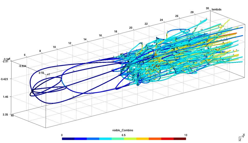
IC-MSQUARE 2020                                                                                                 IOP Publishing
Journal of Physics: Conference Series                         1730 (2021) 012077          doi:10.1088/1742-6596/1730/1/012077

Bifurcation diagram of stationary solutions of the 2D
Kuramoto-Sivashinsky equation in periodic domains.
                      Nikolay M. Evstigneev, Oleg I. Ryabkov
                      Federal Research Center ”Computer Science and Control”, Institute for System Analysis,
                      Russian Academy of Science, 117312, Moscow, pr. 60-letiya Oktyabrya, 9, Russia.
                      E-mail: evstigneevnm@yandex.ru

                      Abstract. The solution tree of the 2D stationary Kuramoto-Sivashinsky equations in the
                      periodic domain is analized using the analytical and numerical methods. The evolution of
                      stationary solutions is considered by constructing the bifurcation diagram. Some bifurcation
                      points on the main solution are found analytically, where secondary bifurcations are analized
                      numerically. The bifurcation diagram is constructed using the deflated pseudo arc-length
                      continuation process that allows one to find both connected and disconnected branches
                      of solutions. The resulting bifurcation diagram is analized and subdivided according to
                      characteristic properties of the solution. Different solution branches are visualized in the physical
                      space.

1. Introduction
The Kuramoto-Sivashinsky equations (KSE) for scalar function u = u(x) : Ω → R is considered
in this paper in the following form:

                                          α (2uux + 2uuy + 4u) + 4 42 u = 0,                                                         (1)

where Ω = (R/2LπZ) × (R/2πZ) is two dimensional torus, L > 0 is the integer stretch factor,
x = (x, y)T is independent variables vector, α is the bifurcation parameter, ()j is the derivative
in the j-direction and 4 is the Laplace operator. The integer constants in     R the equations are
widely used in other papers [1] and the zero mean is assumed in Ω, i.e. Ω udxdy = 0. This
equation is physically relevant in terms of model equations for turbulence as well as chaotic
dynamical systems. Originally, the KSE system was derived independently by G.I.Sivashinsky
[2] in 1977 and Y.Kuramoto [3] in 1978. Physical origin of these equations is the description of
the laminar flame propagation and the description of chaos in the Belousov–Zabotinskii reaction
in three dimensions. These equations also describe dynamics of thin liquid film flows down
inclined plane [4]. It was later used as one of the model equations for chaotic behaviour in PDEs
subject to super-diffusivity. The mathematical study of these equations as well as the analysis of
their inertial manifold are considered in [5, 6]. The analysis of these equations for the 1D spatial
case was studied extensively in many papers, including mathematical and numerical nonlinear
analysis, e.g. [7, 8, 9, 10] and other papers cited within. It was proven that these equations
have a unique smooth solution that has a continuous dependence on the initial conditions. A
global reduction to the approximate inertial manifold for the 1D KSE in periodic domain is
considered in [1], where bifurcations of stationary solutions are analysed. The same results
              Content from this work may be used under the terms of the Creative Commons Attribution 3.0 licence. Any further distribution
              of this work must maintain attribution to the author(s) and the title of the work, journal citation and DOI.
Published under licence by IOP Publishing Ltd                          1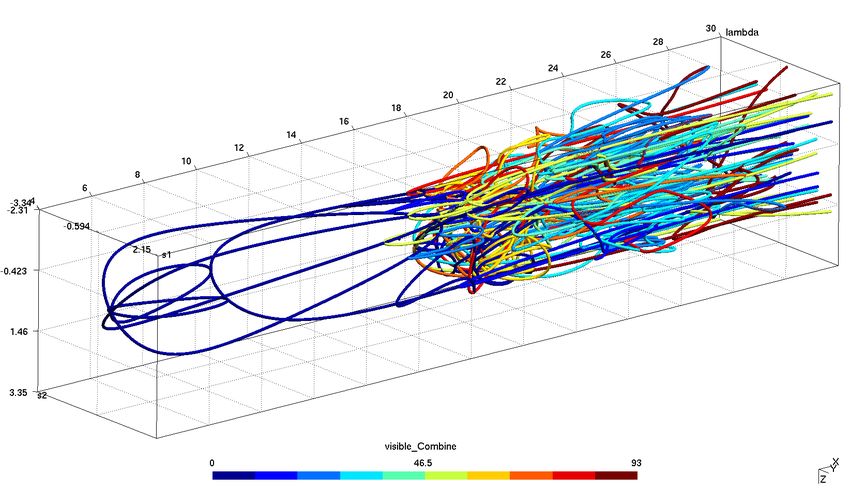
IC-MSQUARE 2020 IOP Publishing
Journal of Physics: Conference Series 1730 (2021) 012077 doi:10.1088/1742-6596/1730/1/012077
were obtained in [11] using computer assisted rigorous computations. It is shown that multiple
nontrivial stationary solutions bifurcate from the main stationary trivial solution at certain
integer points in the parameter space and the kernel dimension of the linearized operator at
these points is greater than unity (higher order degeneration). This results in the formation
of multiple solutions at these bifurcation points by pitchfork bifurcations. The stability loss
of these stationary solutions leads to the occurrence of a two-dimensional local attractor. This
attractor contains all periodic functions of time. Spatially inhomogeneous case gives rise to more
complicated attractors. The bifurcation analysis of periodic solutions indicated the existence of
Feigenbaum and Sharkovskii sequences of bifurcations leading to the chaotic regimes.
The 2D case is still in the field of intense study. It was shown in [12] that only locally
integrable stationary solutions of the 2D KSE are constant values on infinite domain. The
analytical results include [13] the boundness of the solution in the L2 (Ω0 ) ∩ L∞ (t) norm for
unstationary equations (the ones that include the term ut in (1)), where Ω0 = [0, Lπ] × [0, π]
with L > 1 and 0 < < 1. The analyticity for the 2D KSE on the torus Ω for L = 1 is considered
in [14]. It is shown that small solutions exist for all time if there are no linearly growing modes,
proving also in this case that the radius of analyticity of solutions grows linearly in time. For the
genral case the estimates are obtained in terms of mild solutions in L2 (Ω) and H s , 0 ≤ s ≤ 5/3
norms for some finite time T that depends on the regularity of the intial conditions and the
number of linearly growing modes. Authors know of no improvements of this result.
The bifurcation analysis of the trivial solution for the 2D KSE for L = 1 is performed in [15].
It is shown that for wave numbers (j, k) = {(1, 1); (1, 2); (2, 1)} of the Fourier representation of
(1) there exist nontrivial branches and the null-space of the linearized operator has dimensions
two and four. The bifurcated nontrivial solutions are stable at least in the infinitesimal positive
parameter segment at the bifurcation point. The detailed numerical analysis of the non-
stationary 2D KSE is performed in [16] for three different cases: L = 1, L = 10 and somewhat
L >> 1. The statistics of chaotic solutions is considered and the solutions are classified where the
trivial solution is unstable and the long-time dynamics is completely two-dimensional. Various
paths to chaos are observed that are not through period doubling, unlike in the 1D KSE case.
However, a detailed numerical analysis of the stationary solutions of the 2D KSE is not considered
up until now. The authors used (1) as benchmark model problem to tune the deflation pseudo
arc-length continuation method but didn’t find obtained analysis of stationary solutions. This
paper is an attempt to present such analysis.
The paper is laid out as follows. First, the analytical analysis of stationary bifurcations of the
trivial solution is considered. The numerical results are summarized to the bifurcation diagram
on different solution representation functions and various branches are analysed. This follows by
the conclusion. The obtained results also demonstrate the capabilities of the developed software
regarding deflated continuation process.
2. Bifurcation points on the main solution
For periodic
P domain the equation (1) is transfered to the Fourier domain with the ansatz
u(x) = {j,k}∈Z2 ûj,k ei(jx/L+ky) , û0,0 = 0 and û−j,−k = (ûj,k )∗ , due to reality condition that
results in the following discrete infinite dimensional operator:
X l 1 2
F (û, α) = −α 2 i ûl,m ûl−j,m−k + mûl,m ûl−j,m−k − 2
j + k 2 ûj,k −
L L
{l,m}∈Z2 (2)
1 4 2
−4 4
j + 2 j 2 k 2 + k 4 ûj,k = 0, ∀{j, k} ∈ Z2 ,
L L
ˆ = ûj,k = 0 as a trivial solution.
with u0
2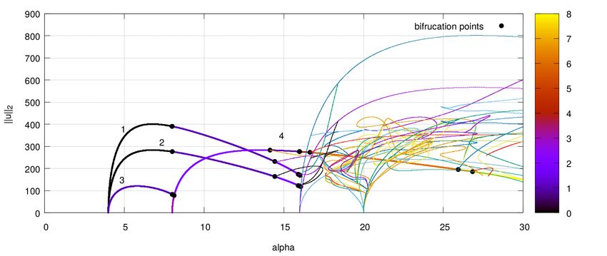
IC-MSQUARE 2020 IOP Publishing
Journal of Physics: Conference Series 1730 (2021) 012077 doi:10.1088/1742-6596/1730/1/012077
One can immediately observe, that the linear operator Fu (û) defined as:
1 2 2 1 4 2 2 2 4
Fu (û)v̂ := α j +k −4 j + 2j k + k v̂j,k −
L2 L4 L
X l
l
(3)
−2iα v̂l,m ûl−j,m−k + mv̂l,m ûl−j,m−k + ûl,m v̂l−j,m−k + mûl,m v̂l−j,m−k ,
2
L L
{l,m}∈Z
∀{j, k} ∈ Z2 ,
ˆ has eigenvalues λj,k = α(j 2 /L2 + k 2 ) − 4(j 2 /L2 + k 2 )2 and eigenvectors
for the trivial solution u0
cos(jx/L ± ky), sin(jx/L ± ky). Hence the possible bifurcation points of the trivial solution
are those points, where αj,k = 4(j 2 /L2 + k 2 ). We restrict ourselves to the solutions that are
symmetric relative to the central point, hence only imaginary vectors are considered in the used
ansatz. Note, that pure imaginary coefficients are preserved by the equations (2), (3). In this
case the eigenvectors el are sin(jx/L + ky), sin(jx/L − ky) and all solutions lies in the Hilbert
space with the zero mean value, we designate H0 .
2.1. Bifurcations for L = 1, α = 4
In this case j = ±1, k = 0 or j = 0, k = ±1. Consider an infinitesimal perturbation with the
magnitude ε and a positive constant β(ε) being applied to the parameter and a solution function:
α = α1 + β(ε)ε2 , (4)
2
X
u= εal el + ε2 v(x, y, ε), (5)
l=1
such that:
v ∈ Sp(e1 , e2 )⊥ ∩ H0 , (6)
P2 2
and l=1 al
= 1, due to the Lyapunov-Schmidt reduction [17]. Plugging these values into the
equation 1 and using the fact (6) one finds the following eight solutions:
u1,2 = ±ε(8 − 2β(0)) sin(x) + O(ε2 ), for a1 = 1, a2 = 0,
u3,4 = ±ε(8 − 2β(0)) sin(y) + O(ε2 ), for a1 = 0, a2 = 1, (7)
√ √
u5,6,7,8 = ε2 (4 + β(0))a1 sin(x) + a2 sin(y) + O(ε3 ), for a1 = ±1/ 2, a2 = ∓1/ 2,
where β(0) is the appropriate constant. We are not interested in the particular constant value,
rather interested in verifying obtained results with the numerical solutions. These solutions
poses a symmetry w.r.t. the main branch. Plugging the Fourier coefficients of these solutions
into the linear operator (3) one sees that solutions u1,2 and u3,4 are stable and u5,6 and u7,8
are unstable. The representation of these solutions is shown in figure 1. The same solutions
at α − 4 ≤ 0.0025 for L = 1 that were obtained numerically during the continuation process
are presented in figure 2. The stability of these solutions is only valid in the vicinity of the
bifurcation point for infinitesimal ε > 0.
2.2. Bifurcations for L = 2, α = 1
In this case j = ±1, k = 0. Using the same approach as before one can obtain two solutions
bifurcating from the trivial one:
ε x x
u1,2 = − sin ± β(0) sin + O(ε2 ), (8)
2 2 2
where one is stable, and the other is not for β(0) > 1.
3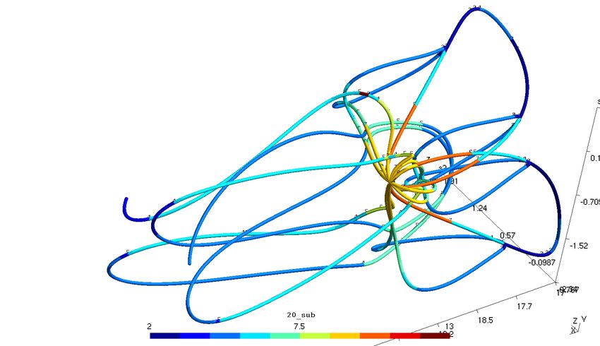
IC-MSQUARE 2020                                                                                                     IOP Publishing
Journal of Physics: Conference Series                            1730 (2021) 012077           doi:10.1088/1742-6596/1730/1/012077

6                                 6                                   6                                 6

5                                 5                                   5                                 5

4                                 4                                   4                                 4

3                                 3                                   3                                 3

2                                 2                                   2                                 2

1                                 1                                   1                                 1

0                                 0                                   0                                 0
    0   1   2   3     4   5   6       0    1   2     3   4   5    6       0   1   2   3   4     5   6       0   1   2   3   4   5   6

Figure 1. Four of the solutions, bifurcating from the trivial zero solution at α = 4, L = 1,
visualization of (7).

Figure 2. Four of the solutions, bifurcating from the trivial zero solution at α−4 ≤ 0.0025, L =
1, obtained through continuation process.

2.3. Bifurcations for L → ∞
In this case α → 0 and for any finite |j| > 0, k = 0 one can observe that a bifurcation occuring
near zero and there are infinitely many bifurcations. These solutions have a form:

                                                   2 sin(x/L)      2β(0) sin(x/L)
                                      u = −ε              2
                                                              − 4ε                + O(ε2 ).                                             (9)
                                                        L                L4
Their stability depends on the constant β(0) which should be found for any particular solution.
However this will involve considering an expansion with parts, having higher degree of ε.

2.4. Bifurcations for L = 1, α = 8
In this case j 2 + k 2 = 2, and j = ±1, k = ±1. This will result in two solutions bifurcating at
this point (not taking symmetric ones into account) of the form:

                                          u1,2 = ε32β0 cos(x ± y) sin(x ± y) + O(ε2 ).                                              (10)

These solutions are unstable and correspond to a1,2 being 1 or 0. Other weights combinations
don’t respect the reduced Lyapunov–Schmidt form. This result can be compared with the results
from [15] where the full set of eigenvalues was considered without symmetry reduction resulting
in four solutions at this point (the case in the paper corresponds to constant in the (1) being 1
and 1 instead of 2 and 4). All solutions are linearly unstable.

2.5. Bifurcations for L > 1, α = 4 1 + L−2

In this case j = ±1, k = ±1 and the bifurcation point α approaches 4 as the value of integer L
approaches infinity. The solutions have a form:

                    u = ∓ε(4 + 4/L2 )1/L(2(cos(x/L − y) ∓ L cos(x/L − y) ± cos(x/L + y)±
                                                                                                                                    (11)
                                          ±L cos(x/L + y))(sin(x/L − y) + sin(x/L + y))) + O(ε2 ),

                                                                          4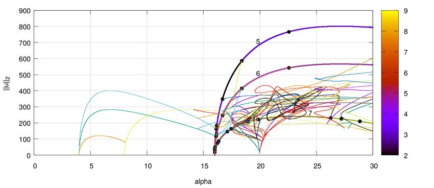
IC-MSQUARE 2020                                                                               IOP Publishing
Journal of Physics: Conference Series            1730 (2021) 012077     doi:10.1088/1742-6596/1730/1/012077

and all these solutions are linearly unstable.
  For the sake of numerical verification we take L = 1 and observe, that the points α,
where j 2 + k 2 = α/4 and {j, k} ∈ Z2 , involve bifurcations of the primary solution, i.e.
α = {4, 8, 16, 20, 32, 36, ...}.

3. Numerical continuation analysis
For the implementation of the numerical analysis we use the earlier developed methods of the
deflated pseudo arc-length continuation being implemented on the multiple graphics processing
units computational architecture [18]. The modified implicitly restarted Arnoldi method
(IRAM) is used [19] with the inexact exponent and inexact exponent shift and inverse matrix
transformations [20]. The analysis is performed according to the following scheme:
  • The set of deflation knots D := {αj }K
                                         j=1 and parameter interval [αs ; αe ] are provided, such,
    that ∀j : αs < αj < αe .
  • Parameters of the numerical schemes and methods are prescribed.
  • The branches and solutions database is initialized.
  • Perform deflation-continuation process according to [18].
  • Use found solutions to perform linear stability analysis using the IRAM.
  • Generate results for each branch and each bifurcation point.
   For this calculation we set L = 1,

                           D = {3.5, 4.5, 5.0, 6.0, 7.5, 8.5, 9.0, 10.5, 12.0, 13.5,
                                                                                                       (12)
                            15.0, 16.5, 18.0, 19.5, 21.0, 22.5, 24.0, 24.5, 25.0},

αs = 3, αe = 30. Hence the continuation is terminated for each branch as soon as the parameter
value reaches 3 or 30. New solution branches, including those that are disconnected from the
main branch, are being found only in deflation knot points according to the methodology in [18].
   The discrete problem is formulated according to (2), where the sums are taken on the finite
ring of integers: 2048 × 2048 Fourier harmonics were used, resulting in N = 2099200 active
degrees of freedom (DOF), the nonlinearity is accounted for using pseudo-spectral approach
with the two thirds de-aliased approach.
   All numerical methods in the deflation-continuation and eigensolver processes execute the
solution of the linear system Ax = b, where linear operator A is Fu (û) from (3) with finite sums.
The system is solved using BiCGStab(L) with the left preconditioner. On each iteration of the
BiCGStab(L) a residual vector r is formed as:

                                                z = b − Ax,
                                                                                                       (13)
                                                    r = Pz,

where the preconditioner P ∼ A−1 is formed as the inverse of the Laplace and biharmonic
operators. It is done easily, since these operators are diagonal matrices in the Fourier space.
The iterations continue, while krk > L .
   All methods for the deflation-continuation are used with Newton-Krylov solvers. The linear
systems are solved up to a small residual reduction followed by the Newton method updates with
the given N . For all deflation-continuation process we set L = 1.0 · 10−2 and N = 1.0 · 10−9 .
The IRAM can also be used with relaxed tolerance for the linear solver, so we set L = 1.0 · 10−4
for the IRAM, and 1.0 · 10−9 for the Ritz vectors norms, see [19]. The points of bifurcation are
found using the bisection method with the parameter value accuracy up to the third significant
digit in mantissa. The parallel performance on multiple GPUs is discussed in [20, 18] and is not
elaborated here.

                                                       5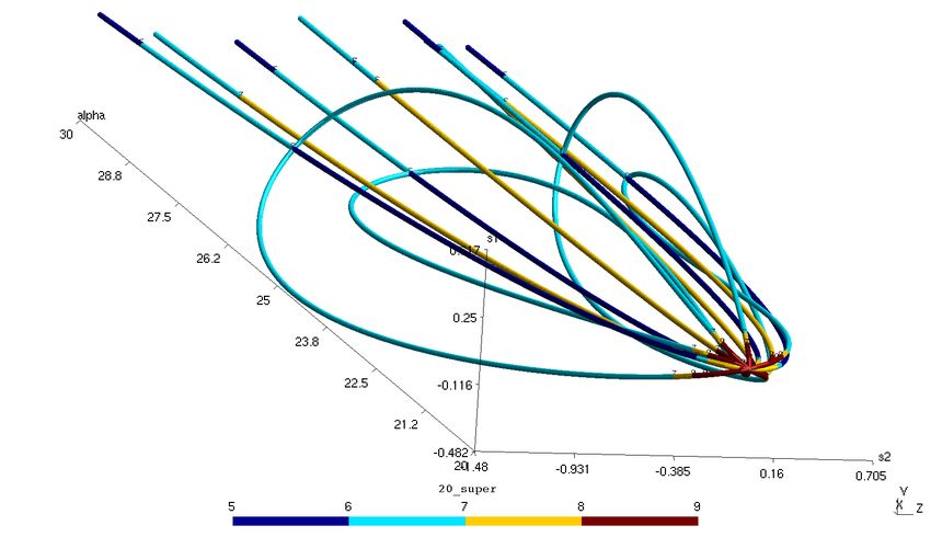
IC-MSQUARE 2020                                                                        IOP Publishing
Journal of Physics: Conference Series       1730 (2021) 012077   doi:10.1088/1742-6596/1730/1/012077

    The solution database is constructed using adaptive strategy for saving intermediate results
on the hard drive, since each solution vector takes roughly 16M B. So only each 50-th solution
is saved on the branch with additional saving solutions when the curve intersects knots (12). We
also save each 20-th solution when the parameter gradient w.r.t. the arc-length has inclination
greater than 1 e.g. at saddle-node bifurcations, and the solution is also saved for each bifurcation
point. Filled database consumes 60GB of hard disk space in binary data file format.

4. Results
From the literature overview and results of the section 2 one can expect a complicated behaviour
of the solutions branches. It is difficult to represent the solutions behaviour adequately in the
2D or 3D space, hence we needed to split the results into different sections. First we present
the full bifurcation diagram. Next we discuss separate branches and bifurcation points. The
following solution representation
                              qPfunctions are used for the solution vector to plot the bifurcation
                         −1/2     N         2
diagrams: kuk2 := N               j=1 |ûj | , s1(u) := u(2π/3, 2π/3), s2(u) := u(2π/5, 2π/3),
s3(u) := u(2π/4, 2π/5) and s4(u) := u(π, 2π/3).

4.1. The whole bifurcation diagram for α ∈ [4, 30]
The whole bifurcation diagram is presented in two figures 3 and 4.

Figure 3.       The whole bifurcation diagram for 4 ≤ α ≤ 30 using s1, s2 functions, colors
represent different branches, totalling 94 curves.

    First, these results represent high complexity of the stationary solutions as the parameter
variates. Figure 4 demonstrates, that the unstable manifold dimension is limited to 13. Although
it is of relatively low complexity (compared, i.e. to the Navier-Stokes equations), the need of
high DOF scheme ensures the fact of the complete scheme resolution, since the unstable manifold
dimension has no link to the approximating linear space DOF. For example a one dimensional
periodic orbit can be expanded into multiple frequencies that would require high DOF scheme.
The analysis of this data as a whole is imposible, so it is conducted as follows: first we analize

                                                  6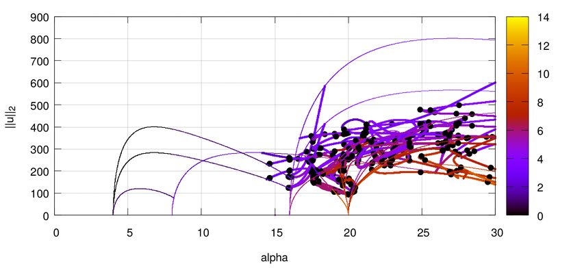
IC-MSQUARE 2020                                                                        IOP Publishing
Journal of Physics: Conference Series       1730 (2021) 012077   doi:10.1088/1742-6596/1730/1/012077

Figure 4.     The whole bifurcation diagram for 4 ≤ α ≤ 30 using s1, s2 functions, colors
represent dimension of the unstable manifold, numbers - points of bifurcation.

all branches that bifurcate from the main zero solution that we call primary. Next, we analize
branches bifurcating from primary branches and disconnected branches, we call these branches
secondary. A trivial zero solution is not traced. We consider k · k2 norms for bifurcation
diagram display and sj, j = {1, 2, 3, 4} representation functions for solution visualization on
branches. Some curves overlap in the k · k2 norm, but this allows a more clear view of a general
picture. All bifurcation points marked in figures correspond to the Hopf bifurcations that are
not analized in this paper, except saddle-node, transcritical and pitchfork bifurcations (both
sub- and supercritical) that result in the change of the unstable manifold dimension. Those are
explicitly discussed.

4.2. Primary branches for α ∈ [4, 8]
The results are presented in figure 5.
   The first bifurcation corresponds to the analytically obtained results (7) at α = 4. We classify
it as symmetry-breaking bifurcation with D4 symmetry group according to the Equivariant
Branching Lemma [21, p.82]. As a result of this bifurcation one has: four steady state solutions
denoted by u1,2,3,4 which are stable near the bifurcation point (these solutions labeled 1 and 2 in
the figure); four steady state solutions denoted by u5,6,7,8 which are unstable near the bifurcation
point (these solutions labeled 3 in the figure). The number of solutions is half of the expected
for D4 group because we only consider solutions symmetric relative to the central point which
corresponds to the quotient group D4 /Z2 . All bifurcation points marked in figure 5 correspond
to the Hopf bifurcations, except one pitchfork bifurcation point near the begining of the curve
4 and one unidentified bifurcation near its ending. This unidentified type of bifurcation will be
discussed later in section 4.4.
   The evolution of four bifurcating solutions is shown in figure 6. Those solutions lose stability
at |α − 8| < 0.005 with the Hopf bifurcation. These branches suffer multiple Hopf bifurcations
resulting in 4 linear operator eigenvalues in the right hand side as α → 16 and two pitchfork

                                                  7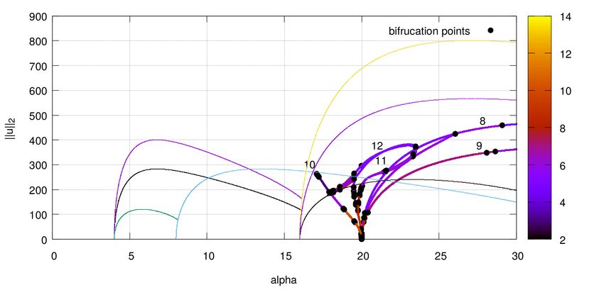
IC-MSQUARE 2020                                                                       IOP Publishing
Journal of Physics: Conference Series      1730 (2021) 012077   doi:10.1088/1742-6596/1730/1/012077

Figure 5. Bifurcation diagram and stability of the primary branches for α ∈ [4, 8] shown in
bold. Curve colors indicate unstable manifold dimension.

Figure 6. Evolution of stable solutions (ones marked with physical space pics) bifurcated at
α = 4 using s3. Colors represent unstable manifold dimension.

bifurcations on each curve that create secondry connecting branches shown on both curves in
figure 5. Bifurcation near |α − 14.4405| < 0.005 is supercritical and near |α − 15.9121| < 0.005
is subcritical.
    The evolution of other four bifurcating solutions is shown in figure 7. These solutions are
initially unstable, also suffer Hopf bifurcations at |α − 8| < 0.005 and end with pitchfork
bifurcations which connect them with primary branches emerging at α = 8.
    The latter solutions, described by (10) bifurcate at α = 8 and are labeled 4 in the figure
5. They suffer multiple Hopf bifurcations, already mentioned pitchfork bifurcations with curves
labeled 3 and six other pitchfork bifurcations - four supercitical and two subcritical. The branch

                                                 8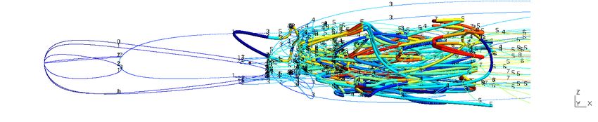
IC-MSQUARE 2020                                                                      IOP Publishing
Journal of Physics: Conference Series     1730 (2021) 012077   doi:10.1088/1742-6596/1730/1/012077

Figure 7. Evolution of unstable solutions (ones marked with physical space pics) at α = 4 in
s4 norm. Colors represent unstable manifold dimension.

Figure 8.      Evolution of the pitchfork bifurcated solutions at α = 8 in s4 norm and four
solutions bifurcated at α = 16 with unstable manifold dimension 2 in s1 norm. Colors represent
unstable manifold dimension.

reaches the termination value of the parameter and is not continued beyond α = 30. Detailed
diagram for these solutions is presented on the left side of the figure 8.

4.3. Primary branches at α = 16
At α = 16 we have j 2 + k 2 = 4 and, hence j = ±2, k = 0 and k = ±2, j = 0, which repeats the
situation for α = 4 but with higher frequency solutions; all bifurcating solutions are unstable

                                               9
IC-MSQUARE 2020 IOP Publishing
Journal of Physics: Conference Series 1730 (2021) 012077 doi:10.1088/1742-6596/1730/1/012077
Figure 9. Bifurcation diagram and stability of the primary branches for α = 16 shown in
bold. Curve colors indicate unstable manifold dimension.
and have greater unstable manifold dimension (two and five) compared to the one at α = 4.
The main branch curves are shown in figure 9 in bold lines labeled as 5, 6 (corresponding to the
four solutions with unstable manifold dimension 2) and 7 (corresponding to the four solutions
with unstable manifold dimension 5) totalling eight curves.
The evolution of solutions on curves 5 and 6 is shown in figure 8, right. These curves suffers 12
secondary pitchfork bifurcations: eight supercritical at |α − 16.18| < 0.005, |α − 16.684| < 0.005
and four subcritical at |α − 16.14| < 0.005. Multiple Hopf bifurcations are observed near the
origin of the primary bifurcation point and are all concentrated at 16 < α ≤ 16.03.
Figure 10. Evolution of four solutions with unstable manifold dimension 5 bifurcated at
α = 16 in s3 norm. Colors represent unstable manifold dimension.
10IC-MSQUARE 2020 IOP Publishing
Journal of Physics: Conference Series 1730 (2021) 012077 doi:10.1088/1742-6596/1730/1/012077
The evolution of other four solutions labeled 7 at α = 16 is shown in figure 10. Apart
from initial symmetry-breaking bifurcation at α = 16, these curves suffer transcritical secondary
bifurcations near |α − 28.8454| < 0.005 resulting in the stability interchange with one of the
secondary branches, four more subcritical pitchfork bifurcations near |α − 17.4135| < 0.005 and
eight more supercritical pitchfork bifurcations near |α − 26.2583| < 0.005. Other points mark
Hopf bifurcations.
4.4. Primary branches at α = 20
Figure 11. Bifurcation diagram and stability of the primary branches for α = 20 shown in
bold. Secondary branches are removed for better visual representation. Curve colors indicate
unstable manifold dimension.
A high order degeneration is observed at α = 20. We have j 2 + k 2 = 5 and, hence
j = ±2, k = ±1 and j = ±1, k = ±2. All bifurcating solutions are unstable. The main
branch curves are shown in figure 11 in bold lines labeled as 8,9 for supercritical and 10 – 12
for subcritical bifurcations. There are 32 curves bifurcating at α = 20, 16 of them, labeled
8,9 are directed in the positive direction of the parameter (supercritical bifurcations) and 16 -
in the negative direction (subcritical bifurcations), labeled 10–12. We interpret this situation
as imposition of four (two supercritical and two subcritical) symmetry-breaking bifurcations
analogous to the ones occuring at α = 4 and α = 16, however, another interpretations might
be possible. The visual representation of these curves is difficult, so 3D visualization is used.
Curves 8, 9 are presented in figure 12.
The results indicate that there are 4 looped curves clearly visible in figure 12. The curves
are formed by subcritical pitchfork bifurcations at |α − 26.0597| < 0.005 and are terminated
at α = 20 with supercritical symmetry-breaking bifurcations discussed above. The evolution of
solutions on these supercritical curves is presented in figure 13. One can observe that most of
these solutions are formed by eigenvectors {sin(2x ± y), sin(x ± 2y)}.
Subcritical curves, bifurcated from α = 20 are presented in figure 14. One can also observe
four loops that are formed by symmetry-breaking and pitchfork bifurcations. A better insight
into the topological structure of solutions can be view in figure 15, where all curves are projected
11IC-MSQUARE 2020 IOP Publishing
Journal of Physics: Conference Series 1730 (2021) 012077 doi:10.1088/1742-6596/1730/1/012077
Figure 12. 3D representation of 16 supercritically bifurcated solutions at α = 20 in coordinates
s1, s2. Colors represent unstable manifold dimension.
onto the s1α plane that respects symmetry of solutions. The curves in the figure are colored
according to the curve classes. Curves 2 are formed by the supercritical bifurcation near
|α − 17.9025| < 0.005 of curves 5. Then the curves 2 suffer three saddle-node bifurcations
in 19.47 < α < 19.53, followed by the subcritical bifurcation at α = 20. Curves 5 apart
from noticed bifurcations and several Hopf bifurcations are initiated at |α − 17.02| < 0.005 by
saddle-node bifurcations and again terminated at α = 20 by the above mentioned subcritical
bifurcation.
Curves 3 and 4 are entangled in a complicated manner. Both curves bifurcate subcritically
at α = 20, followed by multiple turning points (saddle-node bifurcations) that can be observed
in figures 15.
Curves 3 are formed by two unidentified bifurcations from the curves 4 near |α − 17.9025| <
0.005 in such manner, that the curves 4 increase the unstable manifold dimension by one, which
can be seen in figure 14. The problem with classification of these bifurcations is that there
are seemingly no second (paired) branches starting from bifurcation points. This situation is
somewhat similar to the one depicted in [22, p.437] on figure 4.5 and called “mixed-mode”,
connecting different primary branches. However, this analogy could be just visual coincidence
and some further investigation is required. As the result, all curves, but one, entering the
knot at α = 20 are returning trajectories. However, these trajectories form an unstable
manifold of higher dimension near the knot. Part of these bifurcations are due to the secondary
branches connecting the primary, that will be discussed later. The visualization of all subcritical
trajectories that bifurcate at α = 20 is shown in figure 16.
4.5. Secondary branches at 4 < α ≤ 30
Secondary branches of solutions are considered in this subsection that are either formed
by bifurcations on the primaty branches, or by disconnected from the primary branches
separate bifurcations. All secondary bifurcations are presented in figure 17 in bold lines. The
12IC-MSQUARE 2020 IOP Publishing
Journal of Physics: Conference Series 1730 (2021) 012077 doi:10.1088/1742-6596/1730/1/012077
detail analysis of all secondary branches is next to impossible but one can introduce general
classification and describe these branches per class.
The first class contains branches that connect at least one primary branch with other
branches. Such curves are usually formed by above mentioned unidentified unpaired bifurcations
on primary branches. These curves are not closed meaning that these curves contain at least
two such bifurcations at each end. Examples of such curves are presented in figure 18
The second class contains branches that connect at least one primary branch with other
branch and are closed. These branches are usually formed by a pair of pitchfork bifurcations -
one subcritical and the other is supercritical. Examples of these curves are presented in figure
19.
The third class is a subclass of the first two. It contains curves form class 1 or class 2 that
were interrupted during the continuations process and cannot be classified. Those curves are
presented in figure 20
The final, forth class contains four curves that were found during the deflation process and
have no direct connection to other branches. Curves of this type are formed by saddle-node
bifurcations at |α − 18.2725| < 0.005 and |α − 19.5075| < 0.005. Other bifurcations on these
solutions are Hopf bifurcations, thus these solutions have no connection to the main branch.
The unstable manfold dimension on these solutions changes from 4 to 7 due to these Hopf
bifurcations.
The evolution of all solutions on secondary branches is rich and cannot be demonstrated
in the paper. We can refer the reader to the youtube movie at https://www.youtube.com/
watch?v=xoG9NhSqqfo that contains evolution of all solutions glued togethers, both primary
and secondary.
5. Conclusion
We present results of the bifurcation diagram for the 2D stationary Kuramoto–Sivashinsky
equations for 0 < α ≤ 30. It is shown that the stationary solutions undergo process of
bifurcations that turns out to be very complex as the parameter value increases. We defined
two sets of solution curves: primary, that bifurcated from the main solution and secondary that
bifurcated from other solutions, connected to the primary branch, or disconnected. We found
four disconnected solutions that can be formed by high dimensional saddle-node bifurcations.
The next step in the analysis is the generalization of the deflated pseudo arc-length continuation
method to the periodic orbits.
Acknowledgments
This work was supported by the Russian Foundation for Basic Research (grant No. 18-29-10008
mk).
References
[1] Wallace R and Sloan D M 1995 SIAM Journal on Scientific Computing 16 1049–1070
[2] Sivashinsky G 1977 Acta Astronautica 4 1177 – 1206 ISSN 0094-5765
[3] Kuramoto Y 1978 Progress of Theoretical Physics Supplement 64 346–367
[4] Nepomnyashchii A A 1975 Fluid Dynamics 9 354–359
[5] Jolly M S, Rosa R and Temam R 2000 Adv. Differential Equations 5 31–66
[6] Grujić Z 2000 Journal of Dynamics and Differential Equations 12 217–228
[7] Papageorgiou D and Smyrlis Y 1991 Theoretical and Computational Fluid Dynamics 3 15–42
[8] Krishnan J, Kevrekidis I G, Or-Guil M, Zimmerman M G and Markus B 1999 Computer Methods in Applied
Mechanics and Engineering 170 253 – 275 ISSN 0045-7825
[9] Otto F 2009 Journal of Functional Analysis 257 2188–2245
[10] Kulikov A N and Kulikov D A 2018 Automatic Control and Computer Sciences 52 708–713
[11] Arioli G and Koch H 2010 Archive for Rational Mechanics and Analysis 197 1033–1051
[12] Cao Y and Titi E S 2006 Journal of Differential Equations 231 755–767
13IC-MSQUARE 2020 IOP Publishing
Journal of Physics: Conference Series 1730 (2021) 012077 doi:10.1088/1742-6596/1730/1/012077
[13] Molinet L 2000 Journal of Dynamics and Differential Equations 12 533–556
[14] Ambrose D M and Mazzucato A L 2018 Journal of Dynamics and Differential Equations 31 1525–1547
[15] Changpin L and Zhonghua Y 1998 Applied Mathematics-A Journal of Chinese Universities 13 263–270
[16] Kalogirou A, Keaveny E E and Papageorgiou D T 2015 Proceedings of the Royal Society A: Mathematical,
Physical and Engineering Sciences 471 20140932
[17] Guo S and Wu J 2013 Lyapunov–schmidt reduction Applied Mathematical Sciences (Springer New York) pp
119–151
[18] Evstigneev N M 2019 On the convergence acceleration and parallel implementation of continuation in
disconnected bifurcation diagrams for large-scale problems Communications in Computer and Information
Science (Springer International Publishing) pp 122–138
[19] Evstigneev N M 2017 Implementation of implicitly restarted arnoldi method on MultiGPU architecture with
application to fluid dynamics problems Communications in Computer and Information Science (Springer
International Publishing) pp 301–316
[20] Evstigneev N M 2018 Journal of Physics: Conference Series 1141 012121
[21] Golubitsky M, Stewart I and Schaeffer D G 1988 Singularities and Groups in Bifurcation Theory (Springer
New York)
[22] Golubitsky M and Schaeffer D G 1985 Singularities and Groups in Bifurcation Theory (Springer New York)
14IC-MSQUARE 2020 IOP Publishing
Journal of Physics: Conference Series 1730 (2021) 012077 doi:10.1088/1742-6596/1730/1/012077
Figure 13. Evolution of supercritical solutions, bifurcated at α = 20 using s2 representation
function.
15IC-MSQUARE 2020 IOP Publishing
Journal of Physics: Conference Series 1730 (2021) 012077 doi:10.1088/1742-6596/1730/1/012077
Figure 14. 3D representation of 16 subcritically bifurcated solutions at α = 20 in coordinates
s1, s2. Colors represent unstable manifold dimension.
1 1
0.5
0.5
0
-0.5 0
s1
s1
-1
-0.5
-1.5
-2
-1
-2.5
17 18 19 20 21 22 23 24 19.219.319.419.5 19.619.719.819.9 20 20.1
alpha alpha
2 3 4 5 2 3 4 5
Figure 15. Projection to the s1α plane of all curves that bifurcated subciritcally at
α = 20 (left) and zoom-in near the (0, 20) plane point. Colors represent different curve classes,
bifurcation points are represented by colored dots.
16IC-MSQUARE 2020 IOP Publishing
Journal of Physics: Conference Series 1730 (2021) 012077 doi:10.1088/1742-6596/1730/1/012077
Figure 16. Evolution of subcritical solutions, bifurcated at α = 20 using s1 representation
function.
17IC-MSQUARE 2020 IOP Publishing
Journal of Physics: Conference Series 1730 (2021) 012077 doi:10.1088/1742-6596/1730/1/012077
Figure 17. Bifurcation diagram and stability of the secondary branches shown in bold curves.
Curve colors indicate unstable manifold dimension.
Figure 18. Secondary branches of the first class in s1, s2 coordinates. Colors indicate unstable
manifold dimension on each curve.
18IC-MSQUARE 2020 IOP Publishing
Journal of Physics: Conference Series 1730 (2021) 012077 doi:10.1088/1742-6596/1730/1/012077
Figure 19. Secondary branches of the second class in s1, s2 coordinates. Colors indicate
unstable manifold dimension on each curve.
Figure 20. Secondary branches of the third class in s1, s2 coordinates. Colors indicate
unstable manifold dimension on each curve.
19IC-MSQUARE 2020 IOP Publishing
Journal of Physics: Conference Series 1730 (2021) 012077 doi:10.1088/1742-6596/1730/1/012077
Figure 21. Disconnected solutions (curves of the forth class) location in the bifurcation
diagram in s1, s2 coordinates (left) and evolution of solutions (right).
20You can also read