Algorithm to Convert Signal Interpreted Petri Net models to Programmable Logic Controller Ladder Logic Diagram Models - IAES Core
←
→
Page content transcription
If your browser does not render page correctly, please read the page content below
Indonesian Journal of Electrical Engineering and Computer Science
Vol. 10, No. 3, June 2018, pp. 905~916
ISSN: 2502-4752, DOI: 10.11591/ijeecs.v10.i3.pp905-916 905
Algorithm to Convert Signal Interpreted Petri Net models to
Programmable Logic Controller Ladder Logic Diagram Models
Z. Aspar, Nasir Shaikh-Husin, M. Khalil-Hani
Faculty of Electrical Engineering, Universiti Teknologi Malaysia, Malaysia
Article Info ABSTRACT
Article history: Signal Interpreted Petri Nets (SIPN) modeling has been proposed as an
alternative to Ladder Logic Diagram (LLD) modeling for programming
Received Jan 20, 2018 complex programmable logic controllers (PLCs) due to its high level of
Revised Mar 17, 2018 abstraction and functionalities. This paper proposes an algorithm to
Accepted Mar 31, 2018 efficiently convert existing SIPN models to their LLD models equivalences.
In order to automate and speed up the conversion process, matrix calculation
approach is used. A complex SIPN model was used to show that existing
Keywords: conversion technique must be expanded in order to cater for a more complex
SIPN models.
Conversion
Ladder Logic Diagram
Petri Net
Programmable Logic Controller
Copyright © 2018 Institute of Advanced Engineering and Science.
All rights reserved.
Corresponding Author:
Z. Aspar,
Faculty of Electrical Engineering,
Universiti Teknologi Malaysia,
81310 Johor Bahru, Johor, Malaysia.
1. INTRODUCTION
Process control and automation are becoming increasingly complex due to the increases in the
complexity of product specification, shorter design cycles, and shorter product life cycles. To speed up LLD
processing, a new architecture was proposed in [2]. These more demanding systems requirements result in
the need for the conversion of LLD models to high level of abstraction models. A high level of abstraction
modeling paradigm such as Petri Net (PN) [6] or Signal Interpreted Petri Net (SIPN) [16] would allow the
design specification to be defined closer to the product or system requirement while reducing the details of
the lower level implementation. At this abstraction level, a co-design methodology [4] and [7] can be applied
for PLC implementation - either in software, hardware, or a mixture of both. The design trade-offs can be
easily calculated, optimized, and implemented.
The rest of the paper is organized as follows: Section 2 reviews fundamentals of LLD and SIPN.
Related works on PN, LLD and PN-to-LLD conversions are done in Section 3. Several conversion
algorithms have been proposed in [1], [3], [10], [11], [14]-[16] to convert PN to LLD. The analysis of
strengths and limitations are presented in Section 3.2. Section 4 proposes a novel algorithm for SIPN-to-LLD
conversion. Case studies and results for the proposed conversions are discussed and analyzed in Section 5.
Conclusion is in Section 6.
2. LADDER LOGIC AND PETRI NET: A REVIEW
Both PN and LLD were born in 1960’s but for different reasons. PN was invented by Carl Adam
Petri to study asynchronous nature in communication. Meanwhile, LLD was invented due to the needs to
minimize retraining time by mimicking the existing electromechanical relays when PLC was introduced. As
PN grows with more functionality including as an analysis tool as proposed in [18], [20], and [20], LLDs
Journal homepage: http://iaescore.com/journals/index.php/ijeecs
906 ISSN: 2502-4752
evolves into a very important tool in PLC implementation, research on both areas started to merge together at
the end of 1990’s.
2.1. Ladder Logic Diagram
An LLD models the actual combination of relay contacts. A relay contact or a step in LLD is either
normally closed (NC) such as alarm, or normally open (NO) such as main in Figure 1. They are controlled by
logical inputs and state variables which are represented by labels. When an input triggers the step, the
corresponding relay state changes to the opposite state, i.e., the NC step is turned ON while the NO step is
turned OFF. The combination of NC and NO will affect the Output Coil which corresponds to a relay state.
In any LLD such as in Figure 1, the rungs are connecting the power source represented by the
vertical bar on the left, and the ground represented by the vertical bar on the right. Each rung can be divided
into two parts: at the end of the rungs on the right are the outputs, while the rest on the left are the step inputs.
The combination of the step inputs in a rung is also known as the network input. The combination of all rung
outputs in a LLD represents a state. The state can change if any of the output changes due to changes in any
of the step input. Thus, the LLD state varies depending on the steps combination. The step inputs change
either changes directly from external or physical inputs or due to the feedback from the other rungs outputs.
main safe alarm start Cyclic
1 scan
emgcy stop
2
power
pause
start stop run
3
run
Figure 1. LLD for a simple safety circuit
This LLD implements the synchronous assignments of the Boolean equations as:
start = main • safe • alarm
stop = emgcy + power + pause
run = (start + run) • stop
Further, these output changes can be classified either as synchronous process, sequential process, or
combination of both. Sometimes, the difference is hard to notice without any systematic analysis.
2.1. Signal Interpreted Petri Net
Signal Interpreted Petri Nets (SIPN) is an extension of Condition/Event Petri Nets which allows the
handling of binary I/O-signals in a well-defined way. They are well suited to design control algorithms for
discrete event systems resulting in languages standardized in IEC 61131-3. SIPN are defined as a 10-tupel
SIPN = {P, T, F, m0, I, O, φ, ω, Ω, v} where {P, T, F, m0} is ordinary Petri Net. To become SIPN, the
extensions are as:
I – input signals, |I| > 0,
φ – Boolean function in I at T,
Ω – output function combines the output ω of all marked places
O – output signals, |O| > 0 and I ∩ O = Ø
ω – a mapping associating evert Place with an output
v – variable definition assigns a numerical data type
Indonesian J Elec Eng & Comp Sci, Vol. 10, No. 3, June 2018 : 905 – 916
Indonesian J Elec Eng & Comp Sci ISSN: 2502-4752 907
For a more formal definition of SIPN, see [1], [5] and [18]. The dynamic Behavior of an SIPN is
given by the firing process defined by four rules:
1. A transition is enabled, if all its pre-places are marked and firing ensures binary marking of all its post-
places.
2. A transition fires immediately, if it is enabled and its firing condition is fulfilled.
3. All transitions that can fire and are not in conflict with other transitions fire simultaneously.
The firing process is iterated until a stable marking is reached (i.e. until no transition can fire
anymore). Since firing of a transition is supposed to take no time, iterative firing is interpreted as
simultaneous, too. For that reason, no changes of input signals may occur during the firing process. After a
new stable marking is reached, the output signals are computed according to the marking and the signal
algebra.
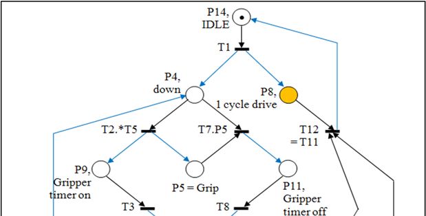
Figure 2. An SIPN model for a robot arm
3. RELATED WORK
Although PN has many advantages over LLD, PLC with LLD as the design entry is the most widely
available in the world. In order to make PN being accepted by existing LLD users, it is important existing
PLC tools and common design techniques can still be reused.
3.1. PN to LLD
There are many works related to PN to LLD conversion e.g. [1], [3], [8]-[16]. Work [9] is an
important survey on all related works on LLD. After some comparison on various techniques in [1], [3], [10],
[11], [14]-[16], the work done in [1] is the best for the job. Their method provides systematic conversion,
isolation from input and output networks, and make the LLD program more readable in order to locate the
fault in LLDs which is a vital issue. These consideration is important to reduce design time and also
debugging and maintenance time. Their method can be extended for SIPN, Timed and Coloured PN.
The conversion process is important due to two important factors: maintaining LLD modeling
paradigm so that users can verify their work using known concept, and validate the PN model that it is
constructed as it was intended to be. Another important thing about their method is the LLD outcome is very
neat and systematic.
Algorithm to Convert Signal Interpreted Petri Net models to Programmable … (Z. Aspar)908 ISSN: 2502-4752
3.2. Previous PN to LLD Conversion
The method proposed in [1] was to identify PN subnets for four different patterns as summarized in
Figure 3. The patterns can be divided into four types in two pairs of set and reset a rung. The set rule is the
condition to activate a rung while the reset rule is the condition to deactivate a rung. The set rules consist of
two general structures known as Type I and Type II. Meanwhile the reset rules consist of two general
structures known as Type III and Type IV. The detail explanation of the rules can be referred in [1].
Figure 3. Types of SET and RESET
4. PROPOSED PN TO LLD CONVERSION
In order to automate and speed up the conversion process, both PN and LLD subnets were analyzed
in their equivalent sub-Incidence Matrices (sub-IM) and sub-Boolean equations (sub-BE) as shown in the
sub-sections 4.1.
4.1. Incident Matrices Method
The output coil in a PLC is denoted by a place, P is renamed as Pj, the k-th feedback input step is Pk,
the n-th step inputs t as T1, T2, to tn as Tn, the analysis on the sub-IM and sub-BE were done on all types of
pattern as illustrated in Figure 3. By referring to previous researcher [1], basically there are four types of
patterns to be identified in the PN. These incudes Type I, Type II, Type III and Type IV. The rule is the value
‘1’ is the output of the transition, (Pj), while the value ‘-1’ is the input of the transition, (Pk). The sub-
incidence matrix and sub-Boolean equation for each Type is discussed:
i. The sub-incidence matrix for Type I:
Pj P1 P2 P3 ... Pk The sub-Boolean equation for Type I can be written as:
T1 1 -1 -1 -1 ... -1 Pj = (P1.P2.P3. ... .Pk).T1
The Boolean equation is generalized as :
Pj Pk .Ti (1)
ii. The sub-incidence matrix for Type II:
P0 P1 P2 P3 ... Pn The sub-Boolean equation for Type II can be written
T1 1 -1 0 0 ... 0 as:
T2 1 0 -1 0 ... 0 P0 = (P1.T1) + (P2.T2) + (P3.T3) + ... (Pn.Tn)
... The Boolean equation is generalized as :
Tn 1 0 0 0 ... -1 Pj Pk .Ti (2)
iii. The sub-incidence matrix for Type III:
P0 P1 P2 P3 ... Pn The sub-Boolean equation for Type III can be written
T1 -1 1 1 1 ... 1 as:
P0 = ... + P0.(Pk + T1)
The Boolean equation is generalized as :
Pj Pj .( Pk Ti ) (3)
Indonesian J Elec Eng & Comp Sci, Vol. 10, No. 3, June 2018 : 905 – 916Indonesian J Elec Eng & Comp Sci ISSN: 2502-4752 909
iv. the sub-incidence matrix for Type IV:
P0 P1 P2 P3 ... Pn The sub-Boolean equation for Type IV can be written
T1 -1 1 0 0 ... 0 as:
T2 -1 0 1 0 ... 0 P0 = + P0.(P1 + T1).(P2 + T2).(P3 + T3). ... .(Pn + Tn)
... The Boolean equation is generalized as :
Tn -1 0 0 0 ... 1 Pj Pj .Pk Ti (4)
Where,
,
The equations are analyzed column by column (k) and row by row (i) starting with the top row
(i=0). These general forms equations are important in the subsequent analysis.
4.2. Custom Transition for LLD
For PLC implementation using LLD model, it is a common practice to have a single step input to
activate or deactivate a rung. In a PN model, the equivalent element to activate or deactivate an output coil is
done by source and sinks transitions respectively. By using them, there is no need to initialize any place with
a token. But this will result in the PN sub-net incomparable with any of pattern types proposed in [1].
Previous analysis shows that the Boolean equation can be automated only if there are value ‘1’ as the
output/input and value ‘-1’ as input/output respectively in a row. The algorithm does not have a solution if in
the row there is only positive numbers or negative numbers as shown in example LLD Type I in Figure 4 and
LLD Type II in Figure 7. The patterns do not exist in the PN model to be converted due to;
a) All positive or all negative coefficients which indicate the source transition or sink transition only.
However, these types of incomplete pattern always exist in PLC applications.
b) Meanwhile, for Type I or Type III does not exist complete pair of transition
c) On the other hand, Type II or Type IV does not have complete pair of input and output transition.
In order to obtain the correct results, PN models should have the complete pair of transition.
Meanwhile, to generate a Boolean equation if there are only value ‘1’ and value ‘0’, or value ‘-1’ and value
‘0’ is by adding a temporary (temp) Place in Petri Nets and it will become wire in the Ladder Logic Diagram.
Type I
Type I PN subnet presented in [1] consists of one transition, one place and one arc as shown in
Figure 4 which has incomplete pair of arc.
Figure 4. A subnet with only one output arc
In order to solve the problem, the incident matrices is used to provide complete pair of input and
output arcs by adding a temporary (Temp) Place in Petri Nets as illustrated in Figure 5. The temporary place
also acts as the current activated place denoted by a token.
Figure 5. A subnet with input and output arc
The equivalent LLD rung by using type I is shown in Figure 6 on the left. Since step Temp is always
ON, the input is always connected and acts as a wire as shown in Figure 6 on the right. This procedure will
Algorithm to Convert Signal Interpreted Petri Net models to Programmable … (Z. Aspar)910 ISSN: 2502-4752
ensure technique in [1] can always be used in a source transition. The similar procedure is also applied for
Type II pattern where the temporary input step will be replaced with a wire.
Temp T1 T1
P1 P1
Figure 6. Final LLD rung for PN subnet Type I
Type III
Type III PN subnet presented in [1] consists of one transition, one place and one arc as shown in
Figure 7 which has incomplete pair of arc.
T1
P1 -1 Incomplete pair
P1 with only an input
arc
T1
Figure 7. A PN subnet with a sink transition
In order to solve this problem, the incident matrices is used to provide a complete pair of the arcs by
adding temporary (Temp) Place in Petri Nets as depicted in Figure 8. The temporary place also acts as the
token destination when the current token is removed from the active place.
P1 T1 Complete pair
with input and
T1 P1 ‐1
output arcs
Figure 8. A subnet to be deactivated by T1
Since it is a reset activity, the equivalent LLD rung by using type III is shown in Figure 9 on the left.
Since step Temp will be OFF when it is activated, the input is always opened and acts as an open connection
as shown in Figure 9 on the right. This procedure will ensure technique in [1] can always be used in a sink
transition. The similar procedure is also applied for Type IV pattern where the temporary input step will be
replaced with an open connection. The technique to use temporary step in generating the equivalent subnet
LLD is important to ensure consistency in the original algorithm in [1]. Once it is consistent, it is easier to
develop the program in a computer.
Figure 9. Final LLD rung for PN subnet Type III
4.3. Critically Unavailable Pattern
In a complicated PN model such as in Figure 2, certain places cannot be converted since the subnets
do not resemble any existing pattern types in [1]. Previous proposed technique in Section 4.2 cannot be
applied since the subnets in Figure 2 are complete subnets. Thus, further adjustment is needed.
Indonesian J Elec Eng & Comp Sci, Vol. 10, No. 3, June 2018 : 905 – 916Indonesian J Elec Eng & Comp Sci ISSN: 2502-4752 911
i. SET
Figure 10 shows a P4 subnet of SIPN from Figure 2. The subnet is going to be activated or set at P5.
This type of structure does not exist in type I, II, III and IV. If the process is automated, the pattern can be
wrongly interpreted as Type III since both look similar. But Type III is for reset.
There is more than a single place connected to transition TP1. If the transition is activated, all the
places connected to the transition will be activated. This also means P9 can be ignored since the place to be
set is P5. Based on this assumption, the subnet has become a Type I pattern.
P4
TP1 = T2.*P5
P9 P5
The subnet IM is as: The subnet IM can be generalized further as:
P4 P5 P9 Ps1 Ps2 ... Psk Pd1 Pd2 ... Pj
TP1 -1 1 1 T -1 -1 -1 1 1 ... 1
Figure 10. A PN subnet from Figure 2 to set
Given one or more source places, Ps and a set of destination places, Pd a single destination place, Pj
can be converted at a time by ignoring the other destination places so that Type I subnet can be generalized
as:
,
The sub-BE can be written as:
Pj Ps1 Ps2 Ps3 ... Psk
a) Pj = (Ps1.Ps2.Ps3. ... .Psk).Ti
Ti 1 -1 -1 -1 ... -1
b) The Boolean equation can be generalized by
And Pd1 = Pd2 = ... Pdn = Pj
following this formula:
Pj Psk .Ti (5)
ii. RESET
Figure 11 shows a subnet of SIPN from Figure 2. The pattern can be wrongly interpreted as Type I
since both look similar. But Type I is for set while this is a reset.
P1
P1 P7
TP2 = T6.P7
T6
P4
P4
Figure 11. A PN subnet from Figure 2 for reset
A transition at T6 is shared with P1 and P7. To disable P1, P7 must also active so that T6 can be
activated. Using transformation technique, one of the place can be combined with the transition and eliminate
the combined place from the subnet as shown in Figure 11 on the right. After the transformation process, the
PN can be categorized as Type III. Now, result from transformation is no longer pure PN, it is known as
signal interpreted petri net (SIPN). The subnet IM is as:
Algorithm to Convert Signal Interpreted Petri Net models to Programmable … (Z. Aspar)912 ISSN: 2502-4752
P1 P4 P7
T6 -1 1 -1
After transformation: The subnet IM can be generalized further as below:
P1 P4
TP2 -1 1 Ps1 Ps2 ... Pj Pd1 Pd2 ... Pdk
Ti -1 -1 -1 1 1 ... 1
Given one or more source places, Ps and a set of destination places, Pd a single destination place, Pj
can be converted at a time by transforming other source places so that Type III subnet can be generalized as:
Pj Pd1 Pd2 ... Pdk The sub-BE can be written as:
TPi -1 1 1 ... 1 a) P0 = ... + P0.(Pk + T1)
Where TPi = Ti . Ps1. Ps2 ... Psn b) The Boolean equation can be generalized by
following this formula
Pj Pj .Pd k Ti (6)
,
iii. SET
Figure 12 shows a subnet of SIPN from Figure 2. The subnet is going to be activated or set at P4.
This type of structure does not exist in type I, II, III and IV. To simplify the subnet, place P8 can be ignored
for the same reason as in Type I. P1 and P7 places are combined to transform into a new subnet as shown in
Figure 12 on the right. The transformation is like in Type III but the subnet is more complicated than the
example in Type III.
P14 P1 P7 P14 TP3 = P1.P7
T1 T6 T1 T6
P8 P4 P4
Figure 12. PN for Type II
After the transformation process, the PN can be categorized as Type II. Without transformation
process, the result becomes wrong. Now, result from transformation is no longer pure PN, it is known as
signal interpreted petri net (SIPN). The original subnet IM is as:
P1 P4 P7 P8 P14 The subnet IM can be generalized further as below:
T1 0 1 0 1 -1 Pj Ps1 Ps2 Ps3 Ps4
T6 -1 1 -1 0 0 Ti 1 0 -1 -1 0
After transformation: Ti + 1 1 -1 0 0 0
TP3 P4 P14 Ti + 2 1 0 0 0 -1
T1 0 1 -1
T6 -1 1 0
Indonesian J Elec Eng & Comp Sci, Vol. 10, No. 3, June 2018 : 905 – 916Indonesian J Elec Eng & Comp Sci ISSN: 2502-4752 913
Given one or more source places, Ps for one transition, Pj can be converted at a time by transforming
other source places so that Type II subnet can be generalized as:
Pj Ps1 TP2 Ps4 The sub-BE can be written as:
Ti 1 0 -1 0 a) P0 = (P1.T1) + (P2.T2) + (P3.T3) + ... (Pn.Tn)
Ti + 1 1 -1 0 0 b) The Boolean equation can be generalized by
Ti + 2 1 0 0 -1 following this formula:
Where TP2 = Ps2. Ps3 ... Psn Pj Pk .Ti (7)
Where:
,
Analyze column by column (k) and row by row (i) starting with the top row (i=0)
iv. RESET
Figure 13 shows a subnet of SIPN from Figure 3. The subnet in Figure 13 is the most complex
subnet due to feedback places and shared transitions at T7.P5. Due to feedback places and shared transitions,
the PN can be seen as Type I due to two input transitions which indicates the SET rung. However, Figure 13
(middle) shows the RESET rung, and the simplification and by eliminating redundant of P5, the Figure 13
(right) gives the correct interpretation of Type IV RESET rung
P4 P4 P5 P4
TT4=T7.P5.P5
T2.P5 T7.P5 T2.P5 T7.P5 T2.P5
P9 P5 P11 P9 P5 P11 P11
TP4 =P9 + P5
Figure 13. PN for Type IV
Original subnet IM is as below:
P4 P5 P9 P11
T2 -1 1 1 0 The subnet IM can be generalized further as below:
T7 -1 -1 0 1
After transformation: Pj Ps1 Ps2 Ps3 Pd1 Pd2 Pd3
P4 TP4 P11 Ti -1 0 0 0 1 1 0
T2 -1 1 0 Ti + 1 -1 -1 0 0 0 0 1
TT4 -1 0 1
Given one or more source places, Ps for one transition and one or more destination places, Pd for one
transition, Pj can be converted at a time by transforming other source and destination places so that Type IV
subnet can be generalized as:
Pj Ps2 Ps3 TP4 Pd3
Ti -1 0 0 0 1
TT4 -1 0 0 0 0
Where TT4 = Ti.Ps1.Ps2….Psn
Ti here is the transition with more than one source places and Ps is the source places.
TP4 = Pd1 + Pd2 + …. Pdn
where Pd here is the destionation places of one transition.
The sub-BE can be written as:
Algorithm to Convert Signal Interpreted Petri Net models to Programmable … (Z. Aspar)914 ISSN: 2502-4752
a) P0 = + P0.(P1 + T1).(P2 + T2).(P3 + T3) . ... . (Pn + Tn)
By using matrix calculation, the results is shown:
Pj Pj . Pk Ti (8)
Where:
,
Figure 14. LLD for robot arm system from SIPN in Figure 2
Indonesian J Elec Eng & Comp Sci, Vol. 10, No. 3, June 2018 : 905 – 916Indonesian J Elec Eng & Comp Sci ISSN: 2502-4752 915
5. RESULT AND ANALYSIS
Figure 2 is a complete and complex SIPN model which is used to control a robot arm. The controller
was developed using a PLC. SIPN modeling was used so that any change can be done quickly using a high
level abstraction. Then, the SIPN model will be converted to the equivalent LLD model using the proposed
algorithm in Section 4.3. Figure 14 shows the equivalent LLD for the SIPN in Figure 2 which was converted
using the proposed algorithm. The LLD model was simulated and tested on an actual robot arm machine to
verify the design. This LLD shows 13 of rungs that indicates the solution for each Place. Looking at equation
(5), (6), (7) and (8), the proposed algorithm used existing equation as in [1]. However, several techniques to
identify unavailable patterns and how to simplify them so that existing formula in [1] can still be reused.
6. CONCLUSION AND FUTURE WORKS
SIPN model for PLC applications are more complicated than the example used in [1]. However,
their PN to LLD conversion method is good enough to be used in an extended work for a more complex
models. This research has shown that in a complete system design, SIPN modeling is useful to model a
complete system and the proposed conversion process can be used by extending the work done previously.
To make the extension work more easily being adopted, and to avoid using two different set of formulas, the
formulas used in previous work were expanded so that the proposed algorithm can be used in both simple and
complex SIPN models. The proposed algorithm also ensures there is only a single set of formulas to be used
at any time to reduce software development complexity.
ACKNOWLEDGEMENTS
The authors are grateful to the Ministry of Science, Technology and Innovation (MOSTI), Ministry
of Higher Education (MOHE), and Universiti Teknologi Malaysia for the financial support through the grants
MOSTI 4S003, MOHE KTP R.J130000.7823.4L500 and MOHE PPRN R.J130000.7623.4C086.
REFERENCES
[1] J-L Chirn and D. C. McFarlane, Petri Nets Based Design of Ladder Logic Diagrams, in Control 2000, Cambridge,
UK, September, 2000. 2000, 4.
[2] Zulfakar Aspar and Mohamed Khalil-Hani, Modeling of a Ladder Logic Processor for High Performance
Programmable Logic Controller, Third Asia International Conference on Modeling & Simulation. 25-29 May
2009: Bandung and Bali, Indonesia, 572 – 577.
[3] E. R. R. Kato, O. Morandin Jr., P. R. Politano and H. A. Camargo, A modular modeling approach for CNC
machines control using Petri Nets, in Systems, Man, and Cybernetics, 2000 IEEE International Conference on.
2000: Nashville, TN, USA, 3147-3152.
[4] Julio A. de Oliveira Filho, Manoel E. de Lima, Paulo Romero Maciel, Petri Net Based Interface Analysis for Fast
IP-Core Integration, in Formal Methods and Models for Co-Design, 2003. MEMOCODE '03. Proceedings. First
ACM and IEEE International Conference on. 2003, 34- 42.
[5] Zuberek, W.M., Throughput Analysis in Timed Petri Nets, in Circuits and Systems, 1992., Proceedings of the 35th
Midwest Symposium on. 1992: Washington, DC, USA, 1576-1580.
[6] Patrick Rokyt, Wolfgang Fengler, and Thorsten Hummel, Electronic System Design Automation using High Level
Petri Nets, in Workshop for Hardware Design and Petri Nets. 1998: Lisboa, 129-138.
[7] Manoel E. Lima, Abel G. S. Filho, Paulo Sérgio B. Nascimento and Paulo Maciel, A reconfigurable codesign
methodology for switching context applications based on Petri net, in 2002 Advanced Simulation Technologies
Conference. 2002: San Diego, California, 8.
[8] Gi BumLee, Han ZanDong, and Jin S. Lee, Automatic generation of Ladder Diagram with control Petri Net.
Intelligent Manufacturing, 2004; 15: 8.
[9] Shih Sen Peng and Meng Chu Zhou., Conversion between Ladder Diagrams and PN in Discrete-Event Control
Design - A Survey, in Systems, Man, and Cybernetics 2001. 2001: Tucson, AZ, USA, 6.
[10] M. Uzam, A.H.J., and N. Ajlouni, Conversion of Petri Net Controllers for Manufacturing Systems into Ladder
Logic Diagrams, in: Proceedings of the IEEE Conference on Emerging Technologies and Factory Automation
(ETFA'96). 1996: Kauai Marriott, Kauai, Hawaii, USA, 649-655.
[11] Mohsen A. Jafari and Thomas O. Boucher, A rule-based system for generating a ladder logic control program from
a high-level systems model. Journal of Intelligent Manufacturing, 1994. 5(2): , 18.
[12] Italia Jimenez, Ernesto Lopez and Antonio Ramfrez, Synthesis of Ladder Diagrams from Petri Nets Controller
Models, in International Symposium on Intelligent Control. 2001: Maxico City, Mexico, 225-230.
[13] Devinder Thapa and Suraj Dangol, and Gi-Nam Wang, Transformation from Petri Nets Model to Programmable
Logic Controller using One-to-One Mapping Technique, in Computational Intelligence for Modeling, Control and
Automation, 2005 and International Conference on Intelligent Agents, Web Technologies and Internet Commerce,
International Conference on. 2005, 228 - 233
Algorithm to Convert Signal Interpreted Petri Net models to Programmable … (Z. Aspar)916 ISSN: 2502-4752
[14] G. L. Burns, and Bopaya Bidanda, "The Use of Hierarchical Petri Nets for the Automatic Generation of Ladder
Logic Programs", Proceedings ESDIPC 94 Conference & Exposition, 169-179, 1994.
[15] Sato, T., and Nose, K., "Automatic Generation of Sequence Control Program via Petri Nets and Logic Tables for
Industrial Applications", Petri Nets in Flexible and Agile Automation, Kluwer Academic Publishers, 1995, 93-108.
[16] Taholakian, A. and Hales, W.M.M., "PN PLC: A methodology for designing, simulating and coding PLC based
control systems using Petri nets", International Journal of Product Research, Jun. 1997, Vol. 35, No. 6, 1743-1762.
[17] Georg Frey, and Lothar Litz, Correctness analysis of petri net based logic controllers, In Proceedings of American
Control Conference, Chicago, Illinois, June 2000, 3165-3166.
[18] Klein, Stéphane, Georg Frey, and Lothar Litz, A petri net based approach to the development of correct logic
controllers, In Proceedings of the 2nd International Workshop on Integration of Specification Techniques for
Applications in Engineering (INT 2002), Grenoble (France).(April 2002), pp. 116-129. 2002.
[19] Hao Yongtao, Zou Zhaoguo and Lou Diming, “Product Spatial Sequence Modeling based on Spatial State
Transition Petri Net of Behavior Flow”, TELKOMNIKA Indonesian Journal of Electrical Engineering, 2013; 11
(9): 5490-5501.
[20] Liu Hongjie, Chen Lijie and Ning Bin, Petri Net-based Analysis of the Safety Communication Protocol,
TELKOMNIKA Indonesian Journal of Electrical Engineering, 2013; 11 (10): 6034-6041.
[21] Haiying Dong and Xionan Li, Fault Diagnosis for Substation with Redundant Protection Configuration Based on
Time-Sequence Fuzzy Petri-Net, TELKOMNIKA (Telecommunication, Computing, Electronics and Control), 2013;
11(2): 231-240.
BIOGRAPHIES OF AUTHORS
Zulfakar Aspar was born in Johor, Malaysia in 1971. He received the B.Sc. in Electrical
Engineering from Case Western Reserve University, USA in 1994. He received his master in
Electrical Engineering from Universiti Teknologi Malaysia, Malaysia in 1999. He completed his
Ph.D. in Electrical Engineering in Universiti Teknologi Malaysia in 2017. Since 1999, he has
been with the Department of Elecronicsl and Computer Engineering (ECE), Faculty of Electrical
Engineering (FKE), Universiti Teknologi Malaysia (UTM) as a lecturer. His research interests
include PLC modeling, microprocessor, digital IC design, FPGA implementation, compiler, and
software development. To enhance his researches, he collaborates with many industries in
respective area.
Nasir Shaikh-Husin is a Senior Lecturer at Dept. of Electronics and Computer Engineering,
Faculty of Electrical Engineering (FKE), Universiti Teknologi Malaysia (UTM). He is presently
Head of Microelectronics Lab at FKE. Nasir obtained his B. Eng. (Electrical) degree from
Lakehead University, Canada in 1985, M.Sc. (Microelectronics) in 1987 from Durham
University, UK and PhD (EE) from UTM in 2008. His research interests are interconnect routing
optimizations and embedded system design.
Mohammed Khalil Bin Mohd Hani received the B.Eng. in electrical from University of
Tasmania, Australia in 1978. Then, he obtained the M.Eng. in electrical from Florida Atlantic
University, USA in 1958. Later he completed his Ph.D. in electrical and computer engineering I
Washington State University, USA in 1992. He is currently a Professor in Faculty of Electrical
Engineering, Universiti Teknologi Malaysia. He has been a lecture in Universiti Teknologi
Malaysia since 1985. He was appointed as Associate Professor in 1995 and later appointed as
Professor in 2000. His research interests include digital systems, embedded hardware, FPGA-on-
Chip design, VLSI design, microelectronic and computer architecture.
Indonesian J Elec Eng & Comp Sci, Vol. 10, No. 3, June 2018 : 905 – 916You can also read