Bi-direction Context Propagation Network for Real-time Semantic Segmentation
←
→
Page content transcription
If your browser does not render page correctly, please read the page content below
Bi-direction Context Propagation Network for Real-time Semantic Segmentation

                                                                 Shijie Hao1      Yuan Zhou1,2          Yanrong Guo1           Richang Hong1
                                                                                        1
                                                                                            Hefei University of Technology
                                                                                        2
                                                                                            2018110971@mail.hfut.edu.cn

                                                                Abstract
arXiv:2005.11034v3 [cs.CV] 2 Jun 2020

                                            Spatial details and context correlations are two types of
                                        important information for semantic segmentation. Generally,
                                        shallow layers tend to contain more spatial details, while
                                        deep layers are rich in context correlations. Aiming to keep
                                        both advantages, most of current methods choose to forward-
                                        propagate the spatial details from shallow layers to deep
                                        layers, which is computationally expensive and substantially
                                        lowers the model’s execution speed. To address this problem,
                                        we propose the Bi-direction Context Propagation Network
                                        (BCPNet) by leveraging both spatial and context information.
                                        Different from the previous methods, our BCPNet builds bi-           Figure 1. Illustrations of the previous forward spatial details propa-
                                        directional paths in its network architecture, allowing the          gation and our backward context propagation mechanism.
                                        backward context propagation and the forward spatial detail
                                        propagation simultaneously. Moreover, all the components
                                        in the network are kept lightweight. Extensive experiments           realize these two key points by 1) keeping high-resolution
                                        show that our BCPNet has achieved a good balance between             feature maps in the network pipeline, and 2) using the di-
                                        accuracy and speed. For accuracy, our BCPNet has achieved            lated convolution [23], respectively [11, 24, 8, 3, 26]. For a
                                        68.4 % mIoU on the Cityscapes test set and 67.8 % mIoU               typical semantic segmentation network, it is well known that
                                        on the CamVid test set. For speed, our BCPNet can achieve            spatial details exist more in the shallow layers, while context
                                        585.9 FPS (or 1.7 ms runtime per image) at 360 × 640 size            information is mainly found in the deep layers. Therefore,
                                        based on a GeForce GTX TITAN X GPU card.                             to enhance the segmentation accuracy via appropriately co-
                                                                                                             operating low-level spatial details and high-level context
                                                                                                             information, these methods try to propagate spatial details
                                                                                                             from shallow layers to deep layers, as shown in Fig.1 (a).
                                        1. Introduction
                                                                                                             However, keeping feature maps of relatively-high resolu-
                                           Semantic segmentation is one of the most challenging              tion in the network tends to bring in higher computational
                                        tasks of computer vision, which aims to partition an image           costs, and thus substantially lowers the execution speed. To
                                        into several non-overlapping regions according to the cate-          quantify the influence of feature resolutions on FLOPs and
                                        gory of each pixel. As its unique role in visual processing,         FPS, we conduct an experiment on the well-known ResNet
                                        many real-world applications rely on this technology such as         [9] framework. For a fair comparison, the last fully con-
                                        self-driving vehicle [17, 20], medical image analysis [7, 6]         nected layer of ResNet is removed. As shown in Fig.2, along
                                        and 3D scenes recognition [28, 19]. Some of these applica-           with the increasing feature resolutions, the model’s FLOPs
                                        tions require high segmentation accuracy and fast execution          substantially increase, and therefore the model’s execution
                                        speed simultaneously, which makes the segmentation task              speed becomes much lower at the same time.
                                        more challenging. In recent years, the research aiming at the           To achieve a good balance between accuracy and speed,
                                        balance between segmentation accuracy and speed is still far         we propose a new method called Bi-direction Context
                                        from satisfactory.                                                   Propagation Network (BCPNet) as shown in Fig.3. Dif-
                                           Generally, there are two key points for obtaining a sat-          ferent from the previous methods that only target to pre-
                                        isfying segmentation: 1) maintaining spatial details, and 2)         serve spatial details, our BCPNet is designed to effectively
                                        aggregating context information. Most of current methods             backward-propagate the context information within the net-
The rest of this paper is organized as follows. First, we
                                                                     introduce the related work in Section 2. Then, we provide
                                                                     the details of our method in Section 3 followed by our ex-
                                                                     periments in Section 4. Finally, we conclude the paper in
                                                                     Section 5.

                                                                     2. Related work
Figure 2. Influence of feature resolutions on FLOPS and speed.           In this section, we review the semantic segmentation
“normalized feature resolution” represents the rate between the      methods which are closely related to our research. First,
feature map size and the input image size. “res-50” represents the
                                                                     the methods based on forward propagation of spatial de-
ResNet-50 network. “res-101” represents the ResNet-101 network.
                                                                     tails within the network pipeline are introduced. Then, we
                                                                     introduce the methods focusing on segmentation speed.
work pipeline, as shown in Fig.1 (b). By propagating the             2.1. Methods of forward-propagating spatial details
context information aggregated from the deep layers back-
ward to the shallow layers, the shallow-layer features become           DilatedNet [23] is a pioneering work based on the forward
more context-aware, as exemplified in Fig.4. Therefore, the          spatial detail propagation, which introduces the dilated con-
shallow-layer features can be directly used for the final pre-       volution to enlarge the receptive field through inserting holes
diction. In our method, the key component is the Bi-direction        to convolution kernels. Therefore, some downsampling op-
Context Propagation (BCP) module (Fig.3 (b)), which effi-            erations (like pooling) can be removed from the network,
ciently enhances the context information of shallow layers by        which avoids the decrease of feature resolutions and the loss
building the bi-directed paths, i.e., the top-down and bottom-       of spatial details. Following [23], a large number of methods
up paths. In this way, the need for keeping high-resolution          are proposed, such as [24, 8, 3, 26]. In particular, most of
feature maps all along in the network pipeline is freed, which       these methods pay attention to improving the context repre-
not only facilitates the design of a network with less FLOPs         sentations of the last convolution layer. For example, [26]
and a faster execution speed, but also maintains a relatively        introduces the Pyramid Pooling Module (PPM), in which
high segmentation accuracy. Specifically, the lightweight            multiple parallel average pooling branches are applied to the
BCPNet is designed, which just totally contains about 0.61           last convolution layer, aiming to aggregate more context cor-
M parameters in a typical segmentation task. Extensive ex-           relations. [3] extendes PPM into the Atrous Spatial Pyramid
periments validate that our BCPNet achieves a good balance           Pooling (ASPP) module by further introducing the dilated
between segmentation accuracy and execution speed. For ex-           convolution [23]. By using the dictionary learning, [24]
ample, as for the speed, our BCPNet achieves 585.9 FPS on            proposes EncNet to learn the global context embedding. Re-
360 × 640 input images. Even for 1024 × 2048 input images,           cently, He et al. [8] propose the Adaptive Pyramid Context
our BCPNet still achieves 55 FPS. As for the segmentation            Network (APCNet), in which the Adaptive Context Module
accuracy, our BCPNet has obtained 68.4 % mIoU on the                 (ACM) is built to aggregate pyramid context information.
cityscapes [5] test set and 67.8 % mIoU on the CamVid [2]               Discussion. Aiming to leverage spatial details and con-
test set.                                                            text correlations, the above methods all propose to propagate
   The contributions of this paper can be summarized as              spatial details from shallow layers to deep layers, as shown
following aspects:                                                   in Fig.1 (a). Nevertheless, the forward spatial detail propa-
                                                                     gation within the network pipeline is computationally expen-
   • First, different from the previous methods that only            sive, and substantially lowers the model’s execution speed
     forward-propagate spatial details, we introduce the             (as shown in Fig.2). Therefore, although these methods im-
     backward context propagation mechanism, which en-               prove segmentation accuracy, the balance between accuracy
     sures the feature maps of shallow layers being aware of         and speed is still far from satisfactory. Taking DeepLab [3]
     semantics.                                                      for example, for a 512 × 1024 input image, the model totally
                                                                     needs 457.8 G FLOPs, at the speed of 0.25 FPS only, as
   • Second, we propose the Bi-direction Context Propaga-            shown in Table.1 and Table.2.
     tion Network (BCPNet), which realizes the backward              2.2. Methods focusing on speed
     context propagation with high efficiency by combining
     the top-down and bottom-up paths.                                   Many real-world applications, such as vision-based self-
                                                                     driving systems, require both segmentation accuracy and
   • Third, as a tiny-size semantic segmentation model, our          efficiency. In this context, large research efforts have been
     BCPNet has achieved the state-of-the-art balance be-            paid to speeding up the semantic segmentation while main-
     tween accuracy and speed.                                       taining its accuracy. For example, Badrinarayanan et al. [1]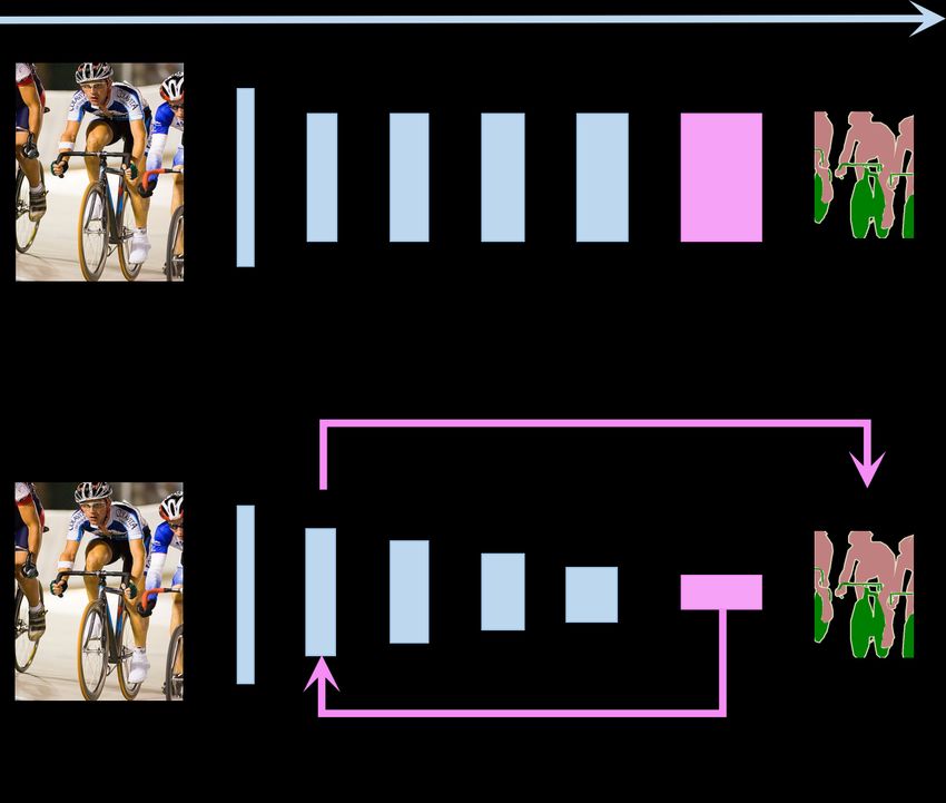
Figure 3. Overview of our BCPNet. “w-sum” represents the weighted sum. “s-conv” represents the separable convolution.

propose SegNet by scaling the network into a small one. Seg-        contains 4.8 M parameters and BiSeNet-2 contains 49 M
Net contains 29.5 M parameters, and can achieve 14.6 FPS            parameters. As for 768 × 1536 input images, BiSeNet-1 in-
on 360 × 640 input images. Moreover, it has achieved 56.1           volves 14.8 G FLOPs and BiSeNet-2 involves 55.3 G FLOPs.
mIoU % on the Cityscapes test set. Paszke et al. [14] pro-          Different from the above methods, we propose to use the
pose ENet by employing the strategy of early downsampling.          context propagation mechanism to construct a real-time se-
ENet contains 0.4 M parameters, and can achieve 135.4               mantic segmentation model.
FPS on 360 × 640 images. Moreover, ENet has achieved
58.3% mIoU on the Cityscapes [5] test set. Zhao et al. [25]         3. Proposed method
propose ICNet by using the strategy of multi-scale inputs
and cascaded frameworks to construct a lightweight net-             3.1. Architecture of BCPNet
work. ICNet contains 26.5 M parameters, and achieves 30.3               As shown in Fig.3, our BCPNet is a variant of encoder-
FPS on 1024 × 2048 input images. Moreover, ICNet has                decoder framework. As for the encoder, we choose the
achieved 67.1 % mIoU on the CamVid [2] test set. Yu et              lightweight MobileNet [16] as our backbone network (Fig.3
al. [22] propose BiSeNet by independently constructing a            (a)). Aiming at an efficient implementation, we do not use
spatial path and a context path. The context path is used to        any dilated convolutions to keep the resolutions of the feature
extract high-level context information, and the spatial path        map in the backbone network. Instead, the feature map is
is used to maintain low-level spatial details. BiSeNet has          fast downsampled to the 1/32 resolution of the input image,
achieved 68.4% mIoU at 72.3 FPS on 768 × 1536 images                which makes the network computationally modest. Since
of the Cityscapes test set. Recently, [10] proposed DFANet          a lightweight network are less capable to learn an accurate
based on the strategy of feature reuse. DFANet has achieved         context representation, our method further aggregate the
71.3 % mIoU at 100 FPS on 1024 × 1024 images of the                 context as in [26] to preserve the segmentation accuracy.
Cityscapes test set. Lo et al. [12] propose EDANet by em-           However, this process is fundamentally different from [26]
ploying an asymmetric convolution structure and dense con-          in two aspects. First, instead of using a parallel manner,
nections, which only includes 0.68 M parameters. EDANet             we aggregate the context by sequentially adopting two max-
can achieve 81.3 FPS based on 512 × 1024 input images.              pooling operations. Second, instead of the average pooling,
Moreover, it still obtains 67.3 % mIoU on the Cityscapes            we use max-pooling to aggregate context information, which
test set.                                                           is empirically useful in our experiments, as shown in Table.5.
    Discussion. Most of the real-time methods concen-               Specifically, we set the kernel size of max-pooling as 3 × 3
trate on scaling the network into a small one, such as              and its stride as 2. Based on the encoder, as shown in Fig.3, a
[1, 14, 25, 10]. However, they ignore the significant role          hierarchy of the feature maps can be obtained. The resolution
of context information in most cases. Although BiSeNet              can be finally condensed into 1/128, which has the global
[22] constructs a spatial path and a context path to learn spa-     perception of the image semantics.
tial details and context correlations respectively, this method         As for the decoder, it contains two parts, i.e., the BCP
is still computationally expensive. For example, BiSeNet-1          module (Fig.3 (b)) and the classifier (Fig.3 (c)). For the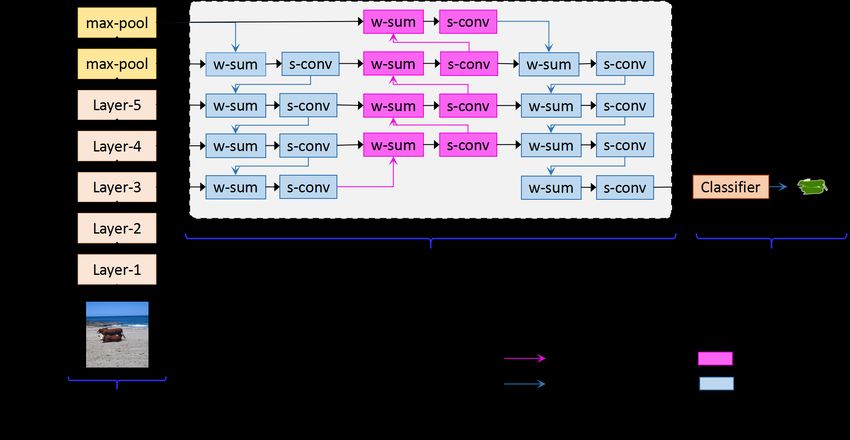
proposed BCP module, we design a bi-directional struc-              map is still aware of object boundaries, and contains much
ture, which enables context information efficiently backward-       less noises. The ablation study in Section.4.4 also validates
propagated to the shallow-layer features, thus making them          the effectiveness of our BCP module.
sufficiently aware of the semantics. Finally, the enhanced
features at the Layer-3 level are sent into the 1 × 1 convolu-      4. Experiments
tional classifier for obtaining the output of the encoder, i.e.
                                                                       In this section, we conduct extensive experiments to vali-
the pixel-wise label prediction of an image.
                                                                    date the effectiveness of our method. First, we compare our
3.2. Details of BCP module                                          method with other methods in terms of the model parameters
                                                                    and FLOPs, implementation speed, and segmentation accu-
    The key component of our BCPNet is the BCP module.              racy. Then, we provide an ablation study for our method.
Aiming to facilitate the segmentation accuracy, we build
the BCP module composed of two top-down paths and one               4.1. Comparison on parameters and FLOPs
bottom-up path. As shown in Fig.3 (b), a top-down path is
                                                                        The number of parameters and FLOPs are important eval-
firstly employed to backward-propagate the context infor-
                                                                    uation metrics for real-time semantic segmentation. There-
mation to shallow layers. Then, a bottom-up path is built
                                                                    fore, in this section, we provide extensive parameters and
to forward-propagate the context and spatial information
                                                                    FLOPs analysis for our method, which is summarized in
aggregated in shallow layers to deep layers again. Finally,
                                                                    Table.1. For a clear comparison, we classify the current re-
another top-down path is employed to backward-propagate
                                                                    lated methods into four categories, i.e., models of large size,
the final context information. In the BCP module, the top-
                                                                    medium size, small size, and tiny size. 1) A large-size model
down path is designed to backward-propagate the context
                                                                    means the network’s parameters and FLOPs are more than
information to shallow layers, while the bottom-up path is
                                                                    200 M and 300 G, respectively . 2) A medium-size model
designed to forward-propagate the spatial information to
                                                                    means the network’s FLOPs are between 100 G and 300 G.
the deep layers. The bi-directional design caters to the key
                                                                    3) A small-size model means the network’s parameters are
concern of a semantic segmentation task, i.e. spatial- and
                                                                    between 1 M and 100 M, or FLOPs are between 10 G and
contextual-awareness. Here, both types of paths have the
                                                                    100 G. 4) A tiny-size model means the network’s parameters
same network structure. Specifically, each layer is composed
                                                                    are less than 1 M, and FLOPs are less than 10 G. According
of two operations, i.e., the separable convolution [4] and the
                                                                    to this, our BCPNet clearly belongs to the category of tiny-
scalar weight sum, which are lightweight. The former one is
                                                                    size model, as it only contains 0.61 M parameters in total,
made up of a point-wise convolution and a depth-wise con-
                                                                    and only involves 4.5 G FLOPs even for the 1024 × 2048
volution. As for the latter, the weighted sum summarizes the
                                                                    input image.
information of neighboring layers by introducing learnable
                                                                        Compared with the small-size models, our BCPNet shows
scalar weights, as shown in Eq.1:
                                                                    a consistently better performance. For example, as for
                                                                    TwoColumn [21], it has about 50 times FLOPs than us. As
                 F = Θl · S l + σl+1 · C l+1                 (1)    for BiSeNet [22], our BCPNet only has about 1.2 % param-
                                                                    eters and 4.6 % FLOPs of BiSeNet-2, and has about 11 %
where S l represents the features from the lth layer (contain-      parameters and 17 % FLOPs of BiSeNet-1. As for ICNet
ing more spatial details), and C l+1 represents features from       [25], our BCPNet only has its 2 % parameters and 16 %
the (l + 1)th layer (containing more context correlations).         FLOPs. As for the two versions of DFANet [10], our FLOPs
The scalars of Θl and σl+1 are learnable weights for S l and        are comparable to them. But we have much less parame-
Cl+1 , respectively.                                                ters, e.g., our BCPNet just has about 13 % parameters of
   Because of the lightweight components, our BCP moldule           DFANet-B and 8 % parameters of DFANet-A.
only contains 0.18 M parameters for a typical segmentation              Compared with other tiny models, our BCPNet still has a
task. However, its effectiveness is satisfying. For example,        better performance. As for ENet [14], although our BCPNet
we visualize two versions of Layer-3 in Fig.4, which are            has more parameters (0.2 M), it just has about 13 % FLOPs
processed with/without the BCP module. We find the feature          of ENet. As for EDANet [12], our parameter number is
map (Fig.4 (b)) without being refined by the BCP module             comparable. But our BCPNet just has about 13 % FLOPs of
contains the rich details, such as boundaries and textures.         EDANet.
However, it is not hlpful for the final segmentation as it is not
                                                                    4.2. Comparison on speed
semantics-aware, since this layer contains too many noises
and lacks sufficient context information. On the contrary,              In this section, we provide the comparison of implemen-
after being refined by the BCP module, the feature maps             tation speed, which is summarized in Table.2.
(Fig.4 (c)) clearly become aware of the regional semantics,             As for the small-size models, our BCPNet presents a con-
such as person, car, and tree. Moreover, the refined feature        sistent faster execution speed. For example, our BCPNet is
Figure 4. Visualization of the feature maps of Layer-3 before and after processed by our BCP module. In particular, as for (b) and (c), red
(blue) color represents the pixel has a higher (lower) response.
Table 1. FLOPs analysis.
Method Params 360 × 640 713 × 713 512 × 1024 768 × 1536 1024 × 1024 1024 × 2048
Large Size
(params > 200M and F LOP s > 300G)
DeepLab [3] 262.1 M - - 457.8 G - - -
PSPNet [26] 250.8 M - 412.2 G - - -
Medium Size
(100G < F LOP s < 300G)
SQ [18] - - - - - - 270 G
FRRN [15] - - - 235 G - - -
FCN-8S [13] - - - 136.2 G - - -
Small Size
(1M < params < 100M or 10G < F LOP s < 100G)
TwoColumn [21] - - - 57.2 G - -
BiSeNet-2 [22] 49 M - - - 55.3 G - -
SegNet [1] 29.5 M 286 G - - - - -
ICNet [25] 26.5 M - - - - - 28.3 G
DFANet-A [10] 7.8 M - - 1.7 G - 3.4 G -
BiSeNet-1 [22] 5.8 M - - - 14.8 G - -
DFANet-B [10] 4.8 M - - - - 2.1 G -
Tiny Size
(params < 1M and F LOP s < 10G)
EDANet [12] 0.68 M - - 8.97 G - - -
ENet [14] 0.4 M 3.8 G - - - - -
Our BCPNet 0.61 M 0.51 G 1.12 G 1.13 G 2.53 G 2.25 G 4.50 G
235.7 FPS faster than TwoColumn [21] based on 512 × 104 faster than DFANet-B on 720 × 960 input images. For
input images. Compared with the two versions of BiSeNet 1024 × 1024 input images, the BCPNet and DFANet-B are
[22], our BCPNet has a clear advantage over them. For ex- comparable, but it is faster than DFANet-A by 16 FPS.
ample, on 360 × 640 input images, our BCPNet is 456.5 FPS As for the tiny-size models, our method still yields better
faster than BiSeNet-2 and 382.4 FPS faster than BiSeNet-1. performances. For example, compared with ENet, our BCP-
When the resolution increases to 720 × 1280, our BCPNet Net is 450 FPS faster on the 360 × 630 input images, and
is 86.9 FPS faster than BiSeNet-2 and 52.5 FPS faster than 88 FPS faster on 720 × 1280 input images. Compared with
BiSeNet-1. Compared with ICNet [25] achieving 30.3 FPS EDANet, on 512 × 1024 input images, our BCPNet is faster
on 1024 × 2048 input images, our BCPNet is still 25 FPS by 69 FPS.
faster than it. Compared with two versions of DFANet [10],
Of note, the results of our model are obtained with a
our BCPNet is 60 FPS faster than DFANet-A, and 20 FPS
GeForce TITAN X GPU card, while the results of othermethods are all obtained with a NVIDIA TITAN X GPU
card, which is slightly better than ours.
4.3. Comparison on accuracy
In this section, we investigate the effectiveness of our
method in terms of accuracy. We first introduce the im-
plement details for our experiments. Then, we compare
the accuracy of our method and the current state-of-the-art
methods on the Cityscapes [5] and CamVid [2] datasets.
4.3.1 Implementation details
Our codes are implemented on the pytorch platform∗ . Fol-
lowing [8, 3], we use the “poly” learning rate strategy, i.e.,
iter power
lr = init lr × (1 − total iter ) . For all the experiments, Figure 5. Visualized segmentation results of our method on the
we set the initial learning rate as 0.1 and the power as 0.9. Cityscapes dataset.
Aiming to reduce the risk of over-fitting, we adopt data aug-
mentation in our experiments. For example, we randomly
flip and scale the input image from 0.5 to 2. We choose the DFANet-B has 7.9 times parameters, and BiSeNet-1 has
Stochastic Gradient Descent (SGD) as the training optimizer, 9.5 times parameters more than ours. As for TwoColumn
in which the momentum is set as 0.9 and weight decay is set [21], whose FLOPs are 50 times than us, the accuracy of
as 0.00001. For the CamVid dataset, we set the crop size and our BCPNet is only 4.5 % lower. Compared with BiSeNet-2
mini-batch as 720 × 720 and 48. For the Cityscapes dataset, [22], whose parameters are 80 times than us, our BCPNet
we set the crop size as 1024 × 1024. Due to the limited GPU has 6.3 % accuracy lower. Despite the lower accuracy, our
resources, we set the mini-batch as 36. For all experiments, BCPNet is much faster than TwoColumn and BiSeNet-2. For
the training process ends after 200 epochs. example, on 512 × 1024 input images, our method is 235
FPS faster than TwoColumn. On 360 × 640 input images,
our method is 456.5 FPS faster than BiSeNet-2.
4.3.2 Cityscapes Compared with the tiny-size models, the BCPNet has a
The Cityscapes [5] dataset is composed of 5000 fine- clear advantage in accuracy. For example, as for ENet [14],
annotated images and 20000 coarse-annotated images. In our method’s accuracy is higher by 10.1 %. As for EDANet
our experiments, we only use the fine-annotated subset. The [12], our method’s accuracy is higher by 1.1 %.
dataset totally includes 30 semantic classes. Following Finally, we visualize some segmentation results of our
[27, 26], we only use 19 classes of them. The fine-annotated method on Fig.5.
subset contains 2975 images for training, 500 images for
validation, and 1525 images for testing. The results on the 4.3.3 CamVid
Cityscapes dataset are summarized in Table.3.
The CamVid dataset [2] is collected from high-resolution
Performance. Compare with the medium-size mod-
video sequences of road senses. This dataset contains 367
els, the accuracy of our method is slightly worse, but still
images for training, 101 images for validation, and 233 im-
achieves an acceptable accuracy level. For example, as for
ages for testing. The dataset totally includes 32 semantic
SQ [18], which has 60 times FLOPs larger than ours, our
classes. Following [25, 10], only 11 classes of them are
BCPNet still obtains 8.6 % higher accuracy. As for FRRM
used in our experiments. The results of our method on the
[15], although it achieves 3.4% accuracy higher than us,
CamVid dataset are summarized in Table.4.
our BCPNet only has 0.5 % of its FLOPs. Moreover, on
Performance. Although our BCPNet contains
512 × 1024 input images, our BCPNet is faster than FRRN
lightweight parameters and FLOPs, it’s accuracy is higher
by 248 FPS. Compared with FCN-8s [13], our BCPNet has
than most of the current state-of-the-art methods. Compared
only 1/120 of its FLOPs, while our accuracy is still by 5.3
with the large-size DeepLab [3], of which the parameters
% higher.
and FLOPs are about 429 and 408 times larger than ours,
Compared with the small-size models, the BCPNet has
the accuracy of our BCPNet is still higher than it by 6.2 %.
achieved comparable accuracy with ICNet [25], DFANet-B
As for the small-size models, our method still has a clear
[10], and BiSeNet-1 [22]. But our BCPNet has much less
advantage of speed-accuracy balance. Compared to SegNet
parameters. For example, ICNet has 43 times parameters,
[1], whose parameters and FLOPs are about 48 and 560
∗ https://pytorch.org times than us, our BCPNet’s accuracy is still higher than itTable 2. Speed analysis for our BCPNet. † represents the method’s speed is calculated on a GeForce TITAN X GPU card. In particular, the
speed of remaining methods is calculated on a NVIDIA TITAN X GPU card. Generally, the NVIDIA TITAN X GPU card is faster than the
GeForce TITAN X GPU card.
360 × 640 512 × 1024 720 × 960 720 × 1280 768 × 1536 1080 × 1920 1024 × 1024 1024 × 2048
Method Params
ms fps ms fps ms fps ms fps ms fps ms fps ms fps ms fps
Large Size
(params > 200M and F LOP s > 300G)
DeepLab [3] 262.1 M - - 4000 0.25 - - - - - - - - - - - -
Medium Size
(100G < F LOP s < 300G)
SQ [18] - - - - - - -- - - - - - - - 60 16.7
FCN-8S [13] - - - 500 2 - -- - - - - - - - - -
FRRN [15] - - - 469 2.1 - -- - - - - - - - - -
Small Size
(1M < params < 100M or 10G < F LOP s < 100G)
TwoColumn [21] - - - 68 14.7 - - - - - - - - - -
BiSeNet-2 [22] 49 M 8 129.4 - - - - 21 47.9 21 45.7 43 23 - - - -
SegNet [1] 29.5 M 69 14.6 - - - - 289 3.5 - - 637 1.6 - - - -
ICNet [25] 26.5 M - - - - 36 27.8 - - - - - - - - 33 30.3
[10] DFANet-A 7.8 M - - 6 160 8 120 - - - - - - 10 100 - -
BiSeNet-1 [22] 5.8 M 5 203.5 - - - - 12 82.3 13 72.3 24 41.4 - - - -
DFANet-B [10] 4.8 M - - - - 6 160 - - - - - - 8 120 - -
Tiny Size
(params < 1M and F LOP s < 10G)
EDANet [12] 0.68 M - - 12.3 81.3 - - - - - - - - - - - -
ENet [14] 0.4 M 7 135.4 - - - - 21 46.8 - - 46 21.6 - - - -
our BCPNet† 0.61 M 1.7 585.9 4 250.4 5.5 181 7.4 134.8 9.8 102.6 18.2 55 8.6 116.2 18.2 55
by a large margin (about 21.1 % higher). Compared with of accuracy. As shown in Table.5, we find that without
ICNet [25], whose parameters and FLOPs are about 43 and our backward context propagration mechanism, the back-
6.2 times larger than us, our BCPNet’s accuracy is higher bone network (containing 0.43 M parameters) only achieves
than it by 0.7 %. Compared with two versions of DFANet 58.891% mIoU on the Cityscapes validation set. By intro-
[10], our BCPNet presents a consistently better performance. ducing the BCP module, the model’s accuracy is increased
For example, as for DFANet-A, whose parameters are about to 67.842 % mIoU (about 9 % higher) with only 0.18 M
12.7 times than us, our method’s accuracy is higher by about additional parameters, which firmly demonstrates the effec-
3.1 %. As for DFANet-B, whose parameters are about 7.8 tiveness of our BCP module. We further investigate the
times than us, our method’s accuracy is higher by about influence of different pooling operations used in context ag-
8.5 %. Compared with two tiny-size models, our method gregation. We find using 3 × 3 max pooling yields a better
has achieved 1.4 % accuracy higher than EDANet [12], performance. When we replace the 3 × 3 max pooling with
and 16.5 higher % than ENet [14]. Of note, although our 3 × 3 average pooling, the performance decreases to 67.311
method’s accuracy is lower than BiSeNet-2 [22] by 0.9 %, % mIoU (abot 0.5 % lower). When we replace the 3 × 3 max
our BCPNet just has about 1.2 % parameters of BiSeNet-1. pooling with 5 × 5 max pooling, the performance decreases
Moreover, compared with lightweight version of BiSeNet-1, to 65.763 % mIoU (about 2 % lower). This can be caused
our BCPNet is more accurate by 2.2 %, and only has about by the mismatch between the (relatively) large kernel size
10 % of its parameters. and the (relatively) small feature resolution. Cropped size
also plays an important role for the final accuracy, which
4.4. Ablation study has been mentioned by [8]. We find using a larger cropped
In this section, we conduct an ablation study to investi- size yields a better performance. For example, when we
gate the influence of our components in BCPNet in terms adopt 1024 × 1024 crop size during the training process, theTable 3. Results of our method on the Cityscapes test set. accuracy, we introduce the backward context propagation
Method Params mIoU mechanism, apart from the forward spatial detail propaga-
Large Size: tion. Both types of the propagation is enabled in the con-
DeepLab [3] 262.1 M 63.1 structed BCP module. To enhance the efficiency, BCPNet
Medium Size: does not keep the high-resolution feature maps all along
SQ [18] - 59.8 the pipeline. In addition, the entire network is constructed
FRRN [15] - 71.8 with lightweight components. Extensive experiments val-
FCN-8S [13] - 63.1
idate that our BCPNet has achieved a new state-of-the-art
Small Size:
balance between accuracy and speed. Due to the tiny size of
TwoColumn [21] - 72.9
BiSeNet-2 [22] 49 M 74.7 our method, we can import the network into mobile devices,
SegNet [1] 29.5 M 56.1 and facilitate several vision-based applications that require
ICNet [25] 26.5 M 69.5 real-time segmentation, such as self-driving and surgery as-
DFANet-A [10] 7.8 M 71.3 sistance.
BiSeNet-1 [22] 5.8 M 68.4
DFANet-B [10] 4.8 M 67.1 References
Tiny Size:
EDANet [12] 0.68 M 67.3 [1] V. Badrinarayanan, A. Kendall, and R. Cipolla. Segnet:
ENet [14] 0.4 M 58.3 A deep convolutional encoder-decoder architecture for
Our BCPNet 0.61 M 68.4 image segmentation. IEEE Transactions on Pattern
Analysis and Machine Intelligence, 39(12):2481–2495,
2017.
Table 4. Results of our method on the CamVid test set.
Method Params mIoU [2] G. J. Brostow, J. Fauqueur, and R. Cipolla. Semantic
Large Size: object classes in video: A high-definition ground truth
DeepLab [3] 262.1 M 61.6 database. Pattern Recognition Letters, 30(2):88–97,
Small Size: 2009.
BiSeNet-2 [22] 49 M 68.7
[3] L.-C. Chen, G. Papandreou, I. Kokkinos, K. Murphy,
SegNet [1] 29.5 M 46.4
ICNet [25] 26.5 M 67.1 and A. L. Yuille. Deeplab: Semantic image segmen-
DFANet-A [10] 7.8 M 64.7 tation with deep convolutional nets, atrous convolu-
BiSeNet-1 [22] 5.8 M 65.6 tion, and fully connected crfs. IEEE Transactions on
DFANet-B [10] 4.8 M 59.3 Pattern Analysis and Machine Intelligence, 40(4):834–
Tiny Size: 848, 2017.
EDANet [12] 0.68 M 66.4
ENet [14] 0.4 M 51.3
[4] F. Chollet. Xception: Deep learning with depthwise
Our BCPNet 0.61 M 67.8 separable convolutions. In Proceedings of the IEEE
Conference on Computer Vision and Pattern Recogni-
tion, pages 1251–1258, 2017.
Table 5. An ablation study of our method on the Cityscapes valida- [5] M. Cordts, M. Omran, S. Ramos, T. Rehfeld, M. En-
tion set. zweiler, R. Benenson, U. Franke, S. Roth, and
Backbone Crop size Pooling BPC Params mIoU B. Schiele. The cityscapes dataset for semantic urban
3 768 × 768 7 7 0.43 M 58.891 scene understanding. In Proceedings of the IEEE Con-
3 768 × 768 3 × 3 max 3 0.61 M 67.842 ference on Computer Vision and Pattern Recognition,
3 768 × 768 3 × 3 avg 3 0.61 M 67.311 pages 3213–3223, 2016.
3 768 × 768 5 × 5 max 3 0.61 M 65.763
3 1024 × 1024 3 × 3 max 3 0.61 M 68.626 [6] Y. Guo, P. Dong, S. Hao, L. Wang, G. Wu, and D. Shen.
Automatic segmentation of hippocampus for longitudi-
nal infant brain mr image sequence by spatial-temporal
hypergraph learning. In International Workshop on
performance can be improved to 68.626 % mIoU. Patch-based Techniques in Medical Imaging, pages
1–8. Springer, 2016.
5. Conclusion
[7] Y. Guo, Y. Gao, and D. Shen. Deformable mr prostate
To achieve a good balance between accuracy and speed segmentation via deep feature learning and sparse patch
in semantic segmentation, we propose a new Bi-direction matching. IEEE Transactions on Medical IDmaging,
Context Propagation Network (BCPNet). To preserve the 35(4):1077–1089, 2015.[8] J. He, Z. Deng, L. Zhou, Y. Wang, and Y. Qiao. Adap- [19] Y. Wang, Y.-T. Huang, and J.-N. Hwang. Monocular
tive pyramid context network for semantic segmen- visual object 3d localization in road scenes. In Pro-
tation. In Proceedings of the IEEE Conference on ceedings of the 27th ACM International Conference on
Computer Vision and Pattern Recognition, pages 7519– Multimedia, pages 917–925, 2019.
7528, 2019. [20] J. Wu, J. Jiao, Q. Yang, Z.-J. Zha, and X. Chen.
[9] K. He, X. Zhang, S. Ren, and J. Sun. Deep resid- Ground-aware point cloud semantic segmentation for
ual learning for image recognition. In Proceedings of autonomous driving. In Proceedings of the 27th ACM
the IEEE Conference on Computer Vision and Pattern International Conference on Multimedia, pages 971–
Recognition, pages 770–778, 2016. 979, 2019.
[10] H. Li, P. Xiong, H. Fan, and J. Sun. Dfanet: Deep [21] Z. Wu, C. Shen, and A. v. d. Hengel. Real-time se-
feature aggregation for real-time semantic segmen- mantic image segmentation via spatial sparsity. arXiv
tation. In Proceedings of the IEEE Conference on preprint arXiv:1712.00213, 2017.
Computer Vision and Pattern Recognition, pages 9522– [22] C. Yu, J. Wang, C. Peng, C. Gao, G. Yu, and N. Sang.
9531, 2019. Bisenet: Bilateral segmentation network for real-time
[11] W. Liu, A. Rabinovich, and A. C. Berg. Parsenet: semantic segmentation. In Proceedings of the Euro-
Looking wider to see better. arXiv preprint pean Conference on Computer Vision (ECCV), pages
arXiv:1506.04579, 2015. 325–341, 2018.
[23] F. Yu and V. Koltun. Multi-scale context aggregation by
[12] S.-Y. Lo, H.-M. Hang, S.-W. Chan, and J.-J. Lin. Ef-
dilated convolutions. arXiv preprint arXiv:1511.07122,
ficient dense modules of asymmetric convolution for
2015.
real-time semantic segmentation. In Proceedings of the
ACM Multimedia Asia on ZZZ, pages 1–6. 2019. [24] H. Zhang, K. Dana, J. Shi, Z. Zhang, X. Wang,
A. Tyagi, and A. Agrawal. Context encoding for se-
[13] J. Long, E. Shelhamer, and T. Darrell. Fully convolu-
mantic segmentation. In Proceedings of the IEEE Con-
tional networks for semantic segmentation. In Proceed-
ference on Computer Vision and Pattern Recognition,
ings of the IEEE Conference on Computer Vision and
pages 7151–7160, 2018.
Pattern Recognition, pages 3431–3440, 2015.
[25] H. Zhao, X. Qi, X. Shen, J. Shi, and J. Jia. Icnet
[14] A. Paszke, A. Chaurasia, S. Kim, and E. Culur- for real-time semantic segmentation on high-resolution
ciello. Enet: A deep neural network architecture images. In Proceedings of the European Conference
for real-time semantic segmentation. arXiv preprint on Computer Vision (ECCV), pages 405–420, 2018.
arXiv:1606.02147, 2016.
[26] H. Zhao, J. Shi, X. Qi, X. Wang, and J. Jia. Pyramid
[15] T. Pohlen, A. Hermans, M. Mathias, and B. Leibe. Full- scene parsing network. In Proceedings of the IEEE
resolution residual networks for semantic segmentation Conference on Computer Vision and Pattern Recogni-
in street scenes. In Proceedings of the IEEE Conference tion, pages 2881–2890, 2017.
on Computer Vision and Pattern Recognition, pages
[27] H. Zhao, Y. Zhang, S. Liu, J. Shi, C. Change Loy,
4151–4160, 2017.
D. Lin, and J. Jia. Psanet: Point-wise spatial attention
[16] M. Sandler, A. Howard, M. Zhu, A. Zhmoginov, and network for scene parsing. In Proceedings of the Euro-
L.-C. Chen. Mobilenetv2: Inverted residuals and linear pean Conference on Computer Vision (ECCV), pages
bottlenecks. In Proceedings of the IEEE Conference 267–283, 2018.
on Computer Vision and Pattern Recognition, pages [28] N. Zhao. End2end semantic segmentation for 3d indoor
4510–4520, 2018. scenes. In Proceedings of the 26th ACM international
[17] M. Siam, S. Elkerdawy, M. Jagersand, and S. Yoga- conference on Multimedia, pages 810–814, 2018.
mani. Deep semantic segmentation for automated driv-
ing: Taxonomy, roadmap and challenges. In 2017 IEEE
20th International Conference on Intelligent Trans-
portation Systems (ITSC), pages 1–8. IEEE, 2017.
[18] M. Treml, J. Arjona-Medina, T. Unterthiner,
R. Durgesh, F. Friedmann, P. Schuberth, A. Mayr,
M. Heusel, M. Hofmarcher, M. Widrich, et al.
Speeding up semantic segmentation for autonomous
driving. In MLITS, NIPS Workshop, volume 2, page 7,
2016.You can also read