Accelerated CNN Training Through Gradient Approximation
←
→
Page content transcription
If your browser does not render page correctly, please read the page content below
Accelerated CNN Training Through Gradient
                            Approximation
                Ziheng Wang                          Sree Harsha Nelaturu                     Saman Amarasinghe
    Department of EECS, Massachusetts               Department of ECE, SRMIST            CSAIL, Massachusetts Institute of
          Institute of Technology                   Kattankulathur, Chennai, India                Technology
          Cambridge, MA, USA                     sreeharsha_murali@srmuniv.edu.              Cambridge, MA, USA
            ziheng@mit.edu                                       in                            saman@mit.edu

Abstract                                                           labor-intensive to set up or maintain. An alternative to using
Training deep convolutional neural networks such as VGG            large computing clusters is to accelerate the computations
and ResNet by gradient descent is an expensive exercise re-        of the gradients themselves. There has been recent effort to
quiring specialized hardware such as GPUs. Recent works            approximate the gradient computation [1, 16, 17, 19]. Other
have examined the possibility of approximating the gradient        recent works have also suggested that the exact gradient might
computation while maintaining the same convergence proper-         not be necessary for efficient training of deep neural networks.
ties. While promising, the approximations only work on rela-       Studies have shown that only the sign of the gradient is nec-
tively small datasets such as MNIST. They also fail to achieve     essary for efficient back propagation [20]. Surprisingly, even
real wall-clock speedups due to lack of efficient GPU imple-       random gradients can be used to efficiently train neural net-
mentations of the proposed approximation methods. In this          works. [10, 12] However, these methods have not been shown
work, we explore three alternative methods to approximate          to result in real wall-clock speedups in training for deep
gradients, with an efficient GPU kernel implementation for         CNNs either due to a lack of efficient GPU implementation or
one of them. We achieve wall-clock speedup with ResNet-20          because the methods only apply to fully connected networks.
and VGG-19 on the CIFAR-10 dataset upwards of 7 percent,              In this work, we hypothesize that we can extend gradient
with a minimal loss in validation accuracy.                        approximation methods to deep CNNs to speed up gradient
                                                                   computations in the training process. We hypothesize that we
Keywords gradient approximation, accelerated training, CNN         can apply these approximations to only a subset of the layers
ACM Reference Format:                                              and maintain the validation accuracy of the trained network.
Ziheng Wang, Sree Harsha Nelaturu, and Saman Amarasinghe. 2019.    We validate our hypotheses on three deep CNNs (2-layer
Accelerated CNN Training Through Gradient Approximation. In        CNN [9], ResNet-20 [7], VGG-19 [15]) on CIFAR-10.
Proceedings of Workshop on Energy Efficient Machine Learning          We summarize our contributions as follows:
and Cognitive Computing for Embedded Applications (EMC2̂, 4th
                                                                       • We present three gradient approximation methods for
Edition). ACM, New York, NY, USA, 5 pages.
                                                                          training deep CNNs, along with an efficient GPU im-
                                                                          plementations for one of them.
1    Introduction                                                      • We explore the application of these methods to deep
Deep convolutional neural networks (CNN) are now arguably                 CNNs and show that they allow for training conver-
the most popular computer vision algorithms. Models such                  gence with minimal validation accuracy loss.
as VGG [15] and ResNet [7] are widely used. However, these
models contain up to hundreds of millions of parameters,           2     Approximation Methods
resulting in high memory footprint, long inference time and
                                                                   In a forward-backward pass of a deep CNN during training, a
even longer training time.
                                                                   convolutional layer requires three convolution operations: one
   The memory footprint and inference time of deep CNNs
                                                                   for forward propagation and two for backward propagation,
directly translate to application size and latency in produc-
                                                                   as demonstrated in Figure 1. We approximate the convolution
tion. Popular techniques based on model sparsification are
                                                                   operation which calculates the gradients of the filter values,
able to deliver orders of magnitude reduction in the number
                                                                   which constitutes roughly a third of the computational time.
of parameters in the network [6]. However, the training of
                                                                   We aim to apply the approximation a quarter of the time
these deep CNNs is still a lengthy and expensive process. Re-
                                                                   across layers/batches. This leads to a theoretical maximum
cent research has attempted to address the training time issue
                                                                   speedup of around 8 percent.
by demonstrating effective training on large scale comput-
ing clusters consisting of thousands of GPUs [21]. However,        2.1   Zero Gradient
these computing clusters are still extremely expensive and
                                                                   The first method passes back zero as the weight gradient of
EMC2̂, 4th Edition, June 23, 2019, Pheonix, AZ                     a chosen layer for a chosen batch. If done for every training
2019.                                                              batch, it effectively freezes the filter weights.
EMC2̂, 4th Edition, June 23, 2019, Pheonix, AZ Ziheng Wang, Sree Harsha Nelaturu, and Saman Amarasinghe
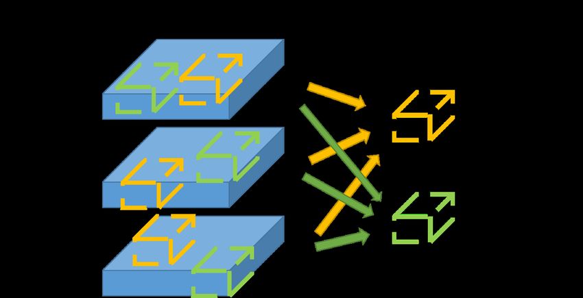
Figure 2. The approximation algorithm illustrated for an
example with two filters and three input elements. For each
filter, we extract a patch from each batch element’s input
activations and accumulate the patches.
top-k magnitude gradient values with an adjustment of the
scaling parameter, a direction of future research. Similar to
Figure 1. Forward and backward propagation through a con-
the random gradient method, we find that we need to scale our
volutional layer during training. Asterisks indicate convolu-
approximated gradient by a factor proportional to the batch
tion operations and the operation in the red box is the one we
size for effective training. In the experiments here, we scale
approximate. 1
them by 128 .
2.2 Random Gradient 2.4 Efficient GPU Implementation
The second method passes back random numbers sampled A major contribution of this work is an implementation of
from a normal distribution with mean 0 and standard devi- the approximated gradient method in CUDA. This is critical
1
ation 128 (inverse of batch size) as the weight gradient of a to achieve actual wall-clock training speedups. A naive Ten-
chosen layer for a chosen batch. Different values in the weight sorflow implementation using tf.image.extract_glimpse does
gradient are chosen independently. Importantly, this is differ- not use the GPU and results in significantly slower training
ent from the random feedback alignment method discussed time. Efficient GPU implementations for dense convolutions
in [10] and [12] as we regenerate the random numbers every frequently use matrix lowering or transforms such as FFT
training batch. We implement this using tf.py_func, where or Winograd. Sparse convolutions, on the other hand, is fre-
np.random.normal is used to generate the random values. This quently implemented directly on CPU or GPU [3, 13]. Here
approach is extremely inefficient, though surprisingly faster we interpret the sparse convolution in the calculation of the fil-
than a naive cuRAND implementation in a custom tensorflow ter gradient as a patch extraction procedure, as demonstrated
operation for most input cases. We are working on a more in Figure 2. The nonzeros in the output specifies patches in
efficient implementation. the input that need to be extracted and averaged.
Our kernel implementation expects input activations in
2.3 Approximated Gradient N HW Ci format and output gradients in NCo HW format. It
The third method we employ is based on the top-k selection produces the output gradient in Co KKCi format. In N HW C
algorithms popular in literature [19]. In the gradient compu- format, GPU global memory accesses from the patch extrac-
tation for a filter in a convolutional layer, only the largest- tions can be efficiently coalesced across the channel dimen-
magnitude gradient value is retained for each output channel sion, which is typically a multiple of 8. Each thread block is
and each batch element. They are scaled according to the sum assigned to process several batch elements for a fixed output
of the gradients in their respective output channels so that channel. Each thread block first computes the indices and
the gradient estimate is unbiased, similar to the approach em- values of the nonzero weight values from the output gradients.
ployed in [18]. All other gradients are set to zero. This results Then, they extract the corresponding patches from the input
1 activations and accumulate them to the result.
in a sparsity ratio of 1 − HW , where H and W are the height
and width of the output hidden layer. The filter gradient is We benchmark the performance of our code against NVIDIA
then calculated from this sparse version of the output gradi- cuDNN v7.4.2 library apis. Approaches such as cuSPARSE
ent tensor with the saved input activations from the forward have been demonstrated to be less effective in a sparse convo-
pass. The algorithm can be trivially modified to admit the lution setting and are not pursued here [3]. All timing metricsAccelerated CNN Training Through Gradient Approximation EMC2̂, 4th Edition, June 23, 2019, Pheonix, AZ are obtained on a workstation with a Titan-Xp GPU and 8 Intel Xeon CPUs at 3.60GHz. All training experiments are conducted in NCHW format, the preferred data layout of cuDNN. As a result, we incur a data transpose overhead of the input activations from NCHW to N HW C. In addition, we also incur a slight data transpose overhead of the filter gradient from Co KKCi to KKCi Co . 3 Evaluation Table 1. Performance comparisons. All timing statistics in We test our approach on three common neural network archi- microseconds. Approx. total column is the sum of the CUDA tectures (2-layer CNN [9], VGG-19 [15] and ResNet-20[7]) Kernel time and the transpose overhead. on the CIFAR-10 dataset. The local response normalization in the 2-layer CNN is replaced by the more modern batch normalization method [8]. For all three networks, we aim to use the approximation methods 25 percent of the time. In this work, we test all three approximation methods sepa- rately and do not combine. On the 2-layer CNN, we apply the selected approximation method to the second convolutional layer every other training batch. On VGG-19 and ResNet-20, we apply the selected approximation method to every fourth Table 2. Training speedup and validation accuracy loss for the convolutional layer every training batch, starting from the approximation methods on 2-layer CNN. Negative speedup second convolutional layer. We start from the second layer indicates a slowdown. because recent work has shown that approximating the first convolutional layer is difficult [1]. This results in four approx- imated layers for VGG-19 and five approximated layers for is expected from the nature of the computations involved: the ResNet-20. We refer to a specification of where and when performance bottleneck of our kernel is the memory intensive to apply the approximation an approximation schedule. For patch extractions, the sizes of which scale with the number the ResNet-20 model, we train a baseline ResNet-14 model of input channels times filter size. Thirdly, we observe that as well. Training a smaller model is typically done in practice in many cases, the data transposition overhead is over fifty when training time is of concern. Ideally, our approximation percent of the kernel time, suggesting that our implementation methods to train the larger ResNet-20 model should result in can be further improved by fusing the data transpose into the higher validation accuracy than the ResNet-14 model. kernel as in SBNet [14]. This is left for future work. 3.1 Performance Comparisons 3.2 Speedup-Accuracy Tradeoffs We compare the performance of our GPU kernel for the ap- Here, we present the training wall-clock speedups achieved proximated gradient method with the full gradient computa- for each network and approximation method. We compare tion for the weight filter as implemented in cuDNN v7.4.2. the speedups against the validation accuracy loss, measured cuDNN offers state-of-the-art performance in dense gradient from the best validation accuracy achieved during training. computation and is used in almost every deep learning library. Validation accuracy was calculated every ten epochs. As afore- Here we demonstrate that our gradient approximation method mentioned, the random gradient implementation is quite in- does yield an efficient GPU implementation that can lead to efficient and is pending future work. The speedup takes into actual speedups compared to cuDNN. account the overhead of defining a custom operation in Ten- We present timing comparisons for a few select input cases sorflow, as well as the significant overhead of switching gra- encountered in the network architectures used in this work in dient computation on global training step. For the 2-layer Table 1. We aggregate the two data transpose overheads of CNN, we are unable to achieve wall-clock speedup for all ap- the input activations and the filter gradients. We make three proximation methods, even the zero gradient one, because of observations. this overhead. (Table 2) However, all approximation methods Firstly, in most cases, the gradient approximation, includ- achieve little validation accuracy loss. The random gradient ing data transposition, is at least three times as fast as the method even outperforms full gradient computation by 0.8%. cuDNN baseline. Secondly, we observe that cuDNN timing For ResNet-20, the approximation schedule we choose scales with the number of input channels times the height and does not involve switching gradient computations. We avoid width of the hidden layer, whereas our approximation kernel the switching overhead and can achieve speedups for both the timing scales with the number of input channels alone. This zero gradient method and the approximated gradient method.
EMC2̂, 4th Edition, June 23, 2019, Pheonix, AZ          Ziheng Wang, Sree Harsha Nelaturu, and Saman Amarasinghe

Table 3. Training speedup and validation accuracy loss for
the approximation methods on ResNet-20. Negative speedup        Table 5. Validation accuracy for different approximation
indicates a slowdown.                                           schedules on ResNet-20. Schedule 1 is the same as presented
                                                                above.

                                                                gradient’s best validation accuracy is within 0.1% of that of
                                                                the full gradient computation. The random gradient method’s
                                                                validation accuracy is in now line with its poor loss curve for
                                                                these two approximation schedules. This suggests that the
Table 4. Training speedup and validation accuracy loss for      random gradient method does not work well for ResNet-20
the approximation methods on VGG-19. Negative speedup           architecture.
indicates a slowdown.
                                                                4   Discussion and Conclusion
                                                                While research on accelerating deep learning inference abounds,
As shown in Table 3, the zero gradient method achieves          there is relatively limited work focused on accelerating the
roughly a third of the speedup compared to training the base-   training process. Recent works such as PruneTrain prune the
line ResNet-14 model. The approximated gradient method          neural network in training, but suffers quite serious loss in
also achieves a 3.5% wall-clock speedup, and is the only        validation accuracy [11]. Approaches such as DropBack [4]
method to suffer less accuracy loss than just using a smaller   and MeProp [16, 19] show that approximated gradient are
ResNet-14. In the following section, we demonstrate that        sufficient in successfully training neural networks but don’t
with other approximation schedules, the approximated gradi-     yet offer real wall-clock speedups. In this work, we study
ent method can achieve as little as 0.1% accuracy loss.         three alternative gradient approximation methods.
   For VGG-19, despite being quicker to converge, the approx-      We are surprised by the consistent strong performance of
imation methods all have worse validation accuracy than the     the zero gradient method. For ResNet-20, for two of the three
baseline method. (Table 4) The best approximation method        approximation schedules tested, the validation accuracy loss
appears to be the random gradient method, though it is ex-      is better than that of a smaller baseline network. Its perfor-
tremely slow due to our inefficient implementation in Ten-      mance is also satisfactory on VGG-19 as well as the 2-layer
sorflow. The other two methods also achieve high validation     CNN. It admits an extremely fast implementation that delivers
accuracies, with the approximated gradient method slightly      consistent speedups. This points to a simple way to potentially
better than the zero gradient method. Both methods are able     boost training speed in deep neural networks, while maintain-
to achieve speedups in training.                                ing their performance advantage over shallower alternatives.
                                                                   We also demonstrate that random gradient methods can
3.3   Robustness to Approximation Schedule                      train deep neural networks to good validation accuracy. For
Here, we explore two new approximation schedules for ResNet-    the 2-layer CNN and VGG-19, this method leads to the least
20, keeping the total proportion of the time we apply the ap-   validation accuracy loss of all three approximation methods.
proximation to 25 percent. We will refer to the approximation   However, its validation accuracy serious lags other methods
schedule presented in the section above as schedule 1. Sched-   on ResNet-20. Naive feedback alignment, where the random
ule 2 applies the selected approximation method every other     gradient signal is fixed before training starts, has been shown
layer for every other batch. Schedule 3 applies the selected    to be difficult to extend to deep convolutional architectures
approximation method every layer for every fourth batch. We     [2, 5] . We show here that if the random gradients are newly
also present the baseline result of the ResNet-14 model.        generated every batch and applied to a subset of layers, they
   As we can see from Table 5, under schedules 2 and 3,         can be used to train deep neural networks to convergence.
both the zero gradient and the approximated gradient method     Interestingly, generating new random gradients every batch
perform well. In fact, for the approximated gradient and the    effectively abolishes any kind of possible “alignment” in the
zero gradient methods the validation accuracy loss is smaller   network, calling for a new explanation of why the network
than schedule 1. Indeed, in schedule 3, the approximated        converges. Evidently, this method holds the potential for an
Accelerated CNN Training Through Gradient Approximation EMC2̂, 4th Edition, June 23, 2019, Pheonix, AZ
extremely efficient implementation, something we are cur- [4] Maximilian Golub, Guy Lemieux, and Mieszko Lis. 2018. DropBack:
rently working on. Continuous Pruning During Training. arXiv preprint arXiv:1806.06949
Finally, we present a gradient approximation method with (2018).
[5] Donghyeon Han and Hoi-jun Yoo. 2019. Efficient Convolutional Neural
an efficient GPU implementation. Our approximation method Network Training with Direct Feedback Alignment. arXiv preprint
is consistent in terms of validation accuracy across different arXiv:1901.01986 (2019).
network architectures and approximation schedules. Although [6] Song Han, Huizi Mao, and William J Dally. 2015. Deep compression:
the training wall clock time speedup isn’t large, the validation Compressing deep neural networks with pruning, trained quantization
accuracy loss is also small. We wish to re-emphasize here and huffman coding. arXiv preprint arXiv:1510.00149 (2015).
[7] Kaiming He, Xiangyu Zhang, Shaoqing Ren, and Jian Sun. 2016. Deep
the small validation accuracy difference observed between residual learning for image recognition. In Proceedings of the IEEE
the baseline ResNet-14 and ResNet-20, leading us to believe conference on computer vision and pattern recognition. 770–778.
that novel training speed-up methods must incur minimal [8] Sergey Ioffe and Christian Szegedy. 2015. Batch normalization: Ac-
validation accuracy loss to be more practical than simply celerating deep network training by reducing internal covariate shift.
training a smaller network. arXiv preprint arXiv:1502.03167 (2015).
[9] Alex Krizhevsky and Geoffrey Hinton. 2009. Learning multiple layers
In conclusion, we show that we can “fool" deep neural of features from tiny images. Technical Report. Citeseer.
networks into training properly while supplying it only very [10] Timothy P Lillicrap, Daniel Cownden, Douglas B Tweed, and Colin J
minimal gradient information on select layers. The approxi- Akerman. 2016. Random synaptic feedback weights support error
mation methods are simple and robust, holding the promise backpropagation for deep learning. Nature communications 7 (2016),
13276.
to accelerate the lengthy training process for state-of-the-art
[11] Sangkug Lym, Esha Choukse, Siavash Zangeneh, Wei Wen, Mattan
deep CNNs. Erez, and Sujay Shanghavi. 2019. PruneTrain: Gradual Structured Prun-
ing from Scratch for Faster Neural Network Training. arXiv preprint
5 Future Work arXiv:1901.09290 (2019).
[12] Arild Nøkland. 2016. Direct feedback alignment provides learning in
Besides those already mentioned, there are several more inter- deep neural networks. In Advances in neural information processing
esting directions of future work. One direction is predicting systems. 1037–1045.
the validation accuracy loss that a neural network would suffer [13] Jongsoo Park, Sheng Li, Wei Wen, Ping Tak Peter Tang, Hai Li, Yi-
from a particular approximation schedule. With such a predic- ran Chen, and Pradeep Dubey. 2016. Faster cnns with direct sparse
convolutions and guided pruning. arXiv preprint arXiv:1608.01409
tor, we can optimize for the fastest approximation schedule (2016).
while constraining the final validation accuracy loss before [14] Mengye Ren, Andrei Pokrovsky, Bin Yang, and Raquel Urtasun. 2018.
the training run. This would remove the need for arbitrarily Sbnet: Sparse blocks network for fast inference. In Proceedings of
selecting an approximation ratio like we did here. We can the IEEE Conference on Computer Vision and Pattern Recognition.
also examine the effects of mingling different approximation 8711–8720.
[15] Karen Simonyan and Andrew Zisserman. 2014. Very deep convo-
methods and integrating existing methods such as PruneTrain lutional networks for large-scale image recognition. arXiv preprint
and Dropback [4, 11]. Another direction is approximating arXiv:1409.1556 (2014).
the gradient of the hidden activations, as is done in meProp [16] Xu Sun, Xuancheng Ren, Shuming Ma, and Houfeng Wang. 2017.
[16]. Finally, we are working on integrating this approach meprop: Sparsified back propagation for accelerated deep learning with
into a distributed training setting, where the approximation reduced overfitting. In Proceedings of the 34th International Conference
on Machine Learning-Volume 70. JMLR. org, 3299–3308.
schedule is now 3-dimensional (machine, layer, batch). This [17] Xu Sun, Xuancheng Ren, Shuming Ma, Bingzhen Wei, Wei Li, Jingjing
approach would be crucial for the approximation methods Xu, Houfeng Wang, and Yi Zhang. 2018. Training simplification
to work with larger scale datasets such as ImageNet, thus and model simplification for deep learning: A minimal effort back
potentially allowing for wall-clock speed-up in large scale propagation method. IEEE Transactions on Knowledge and Data
training. Engineering (2018).
[18] Jianqiao Wangni, Jialei Wang, Ji Liu, and Tong Zhang. 2018. Gradient
sparsification for communication-efficient distributed optimization. In
Acknowledgments Advances in Neural Information Processing Systems. 1306–1316.
[19] Bingzhen Wei, Xu Sun, Xuancheng Ren, and Jingjing Xu. 2017. Mini-
We thank Ajay Brahmakshatriya for helpful advice.
mal effort back propagation for convolutional neural networks. arXiv
preprint arXiv:1709.05804 (2017).
References [20] Will Xiao, Honglin Chen, Qianli Liao, and Tomaso Poggio. 2018.
Biologically-plausible learning algorithms can scale to large datasets.
[1] Menachem Adelman and Mark Silberstein. 2018. Faster Neural Net-
arXiv preprint arXiv:1811.03567 (2018).
work Training with Approximate Tensor Operations. arXiv preprint
[21] Yang You, Zhao Zhang, Cho-Jui Hsieh, James Demmel, and Kurt
arXiv:1805.08079 (2018).
Keutzer. 2018. Imagenet training in minutes. In Proceedings of the
[2] Sergey Bartunov, Adam Santoro, Blake Richards, Luke Marris, Geof-
47th International Conference on Parallel Processing. ACM, 1.
frey E Hinton, and Timothy Lillicrap. 2018. Assessing the scalability
of biologically-motivated deep learning algorithms and architectures.
In Advances in Neural Information Processing Systems. 9368–9378.
[3] Xuhao Chen. 2018. Escort: Efficient sparse convolutional neural net-
works on gpus. arXiv preprint arXiv:1802.10280 (2018).You can also read