Natural Language Processing with Deep Learning CS224N/Ling284 - Christopher Manning Lecture 7: Machine Translation, Sequence-to-Sequence and ...

Natural Language Processing
 with Deep Learning
 CS224N/Ling284

 Christopher Manning
Lecture 7: Machine Translation, Sequence-to-Sequence and Attention

Lecture Plan
Today we will:
1. Introduce a new task: Machine Translation [15 mins], which is a major use-case of
2. A new neural architecture: sequence-to-sequence [45 mins], which is improved by
3. A new neural technique: attention [20 mins]

• Announcements
 • Assignment 3 is due today – I hope your dependency parsers are parsing text!
 • Assignment 4 out today – covered in this lecture, you get 9 days for it (!), due Thu
 • Get started early! It’s bigger and harder than the previous assignments 
 • Thursday’s lecture about choosing final projects

2

Section 1: Pre-Neural Machine Translation

3

Machine Translation
Machine Translation (MT) is the task of translating a sentence x from one language (the
source language) to a sentence y in another language (the target language).

 x: L'homme est né libre, et partout il est dans les fers

 y: Man is born free, but everywhere he is in chains

 – Rousseau
4

The early history of MT: 1950s
• Machine translation research began in the early 1950s on machines less
 powerful than high school calculators
• Foundational work on automata, formal languages, probabilities, and
 information theory
• MT heavily funded by military, but basically just simple rule-based
 systems doing word substitution
• Human language is more complicated than that, and varies more across
 languages!
• Little understanding of natural language syntax, semantics, pragmatics
• Problem soon appeared intractable
1 minute video showing 1954 MT:
https://youtu.be/K-HfpsHPmvw

1990s-2010s: Statistical Machine Translation
 • Core idea: Learn a probabilistic model from data
 • Suppose we’re translating French → English.
 • We want to find best English sentence y, given French sentence x

 • Use Bayes Rule to break this down into two components to be learned
 separately:

 Translation Model Language Model

 Models how words and phrases Models how to write
 should be translated (fidelity). good English (fluency).
6 Learnt from parallel data. Learnt from monolingual data.

1990s-2010s: Statistical Machine Translation
• Question: How to learn translation model ?
• First, need large amount of parallel data
 (e.g., pairs of human-translated French/English sentences)

 The Rosetta Stone Ancient Egyptian

 Demotic

 Ancient Greek

7

Learning alignment for SMT
 • Question: How to learn translation model from the parallel corpus?

 • Break it down further: Introduce latent a variable into the model:

 where a is the alignment, i.e. word-level correspondence between source sentence x
 and target sentence y

8

What is alignment?
Alignment is the correspondence between particular words in the translated sentence pair.

• Typological differences between languages lead to complicated alignments!
• Note: Some words have no counterpart

9 Examples from: “The Mathematics of Statistical Machine Translation: Parameter Estimation", Brown et al, 1993. http://www.aclweb.org/anthology/J93-2003

Alignment is complex
 Alignment can be many-to-one

10 Examples from: “The Mathematics of Statistical Machine Translation: Parameter Estimation", Brown et al, 1993. http://www.aclweb.org/anthology/J93-2003

Alignment is complex
 Alignment can be one-to-many

11 Examples from: “The Mathematics of Statistical Machine Translation: Parameter Estimation", Brown et al, 1993. http://www.aclweb.org/anthology/J93-2003

Alignment is complex
 Alignment can be many-to-many (phrase-level)

12 Examples from: “The Mathematics of Statistical Machine Translation: Parameter Estimation", Brown et al, 1993. http://www.aclweb.org/anthology/J93-2003

Learning alignment for SMT
 • We learn as a combination of many factors, including:
 • Probability of particular words aligning (also depends on position in sent)
 • Probability of particular words having a particular fertility (number of corresponding
 words)
 • etc.
 • Alignments a are latent variables: They aren’t explicitly specified in the data!
 • Require the use of special learning algorithms (like Expectation-Maximization) for
 learning the parameters of distributions with latent variables
 • In older days, we used to do a lot of that in CS 224N, but now see CS 228!

13

Decoding for SMT

 Language Model
 Question:
 How to compute Translation Model
 this argmax?

 • We could enumerate every possible y and calculate the probability? → Too
 expensive!
 • Answer: Impose strong independence assumptions in model, use dynamic
 programming for globally optimal solutions (e.g. Viterbi algorithm).
 • This process is called decoding

14

Decoding for SMT Translation Options
 er geht ja nicht nach hause
 he is yes not after house
 it are is do not to home
 , it goes , of course does not according to chamber
 , he go , is not in at home
 it is
 he will be
 it goes
 Decoding: Find Best Path not
 is not
 does not
 home
 under house
 return home
 he goes do not do not
 is to
 er are geht ja nicht
 following nach hause
 is after all not after
 does not to
 not
 is not
 are not
 is not a

 • Many translation options to choose from
 yes
 – in Europarl phrase table: 2727 matching phrase pairs for this sentence
 – by pruning to the top 20 perhephrase, 202 translationhome
 goes options remain

 are
 does not go home
 Chapter 6: Decoding 8
 it
 to

 Source: ”Statistical Machine Translation", Chapter 6, Koehn, 2009.
 backtrack https://www.cambridge.org/core/books/statistical-machine-translation/94EADF9F680558E13BE759997553CDE5
 from highest scoring complete hypothesis
15

1990s-2010s: Statistical Machine Translation
 • SMT was a huge research field
 • The best systems were extremely complex
 • Hundreds of important details we haven’t mentioned here
 • Systems had many separately-designed subcomponents
 • Lots of feature engineering
 • Need to design features to capture particular language phenomena
 • Require compiling and maintaining extra resources
 • Like tables of equivalent phrases
 • Lots of human effort to maintain
 • Repeated effort for each language pair!

16

Section 2: Neural Machine Translation

17

2014

 (dramatic reenactment)
18

2014 Ne
 u
 Ma ral
 Tra chin
 nsl e
 atio
 n

 MT
 res
 earc
 h (dramatic reenactment)
19

What is Neural Machine Translation?
 • Neural Machine Translation (NMT) is a way to do Machine Translation with a single
 end-to-end neural network

 • The neural network architecture is called a sequence-to-sequence model (aka seq2seq)
 and it involves two RNNs

20

Neural Machine Translation (NMT)
 The sequence-to-sequence model
 Target sentence (output)
 Encoding of the source sentence.
 Provides initial hidden state
 he hit me with a pie 
 for Decoder RNN.

 argmax

 argmax

 argmax

 argmax

 argmax
 argmax

 argmax
 Encoder RNN

 Decoder RNN
 il a m’ entarté he hit me with a pie

 Source sentence (input) Decoder RNN is a Language Model that generates
 target sentence, conditioned on encoding.
 Encoder RNN produces Note: This diagram shows test time behavior: decoder
 an encoding of the output is fed in as next step’s input
 source sentence.
21

Sequence-to-sequence is versatile!
 • Sequence-to-sequence is useful for more than just MT

 • Many NLP tasks can be phrased as sequence-to-sequence:
 • Summarization (long text → short text)
 • Dialogue (previous utterances → next utterance)
 • Parsing (input text → output parse as sequence)
 • Code generation (natural language → Python code)

22

Neural Machine Translation (NMT)
 • The sequence-to-sequence model is an example of a Conditional Language Model
 • Language Model because the decoder is predicting the
 next word of the target sentence y
 • Conditional because its predictions are also conditioned on the source sentence x

 • NMT directly calculates :

 Probability of next target word, given
 target words so far and source sentence x
 • Question: How to train a NMT system?
 • Answer: Get a big parallel corpus…

23

Training a Neural Machine Translation system
 = negative log = negative log = negative log
 * prob of “he” prob of “with” prob of 
 1
 = ' ( = ! + " + # + $ + % + & + '
 
 ()!

 !! !" !# !$ !% !& !'

 Decoder RNN
 Encoder RNN

 il a m’ entarté he hit me with a pie

 Source sentence (from corpus) Target sentence (from corpus)

 Seq2seq is optimized as a single system. Backpropagation operates “end-to-end”.
24

Multi-layer RNNs
• RNNs are already “deep” on one dimension (they unroll over many timesteps)

• We can also make them “deep” in another dimension by applying multiple RNNs
 – this is a multi-layer RNN.

• This allows the network to compute more complex representations
 • The lower RNNs should compute lower-level features and the higher RNNs should
 compute higher-level features.

• Multi-layer RNNs are also called stacked RNNs.

25

Multi-layer deep encoder-decoder machine translation net
[Sutskever et al. 2014; Luong et al. 2015]
 The hidden states from RNN layer i
 are the inputs to RNN layer i+1

 Translation
 The protests escalated over the weekend 
 generated
 0.1 0.2 0.4 0.5 0.2 -0.1 0.2 0.2 0.3 0.4 -0.2 -0.4 -0.3
 0.3 0.6 0.4 0.5 0.6 0.6 0.6 0.6 0.6 0.4 0.6 0.6 0.5
 0.1 -0.1 0.3 0.9 -0.1 -0.1 -0.1 -0.1 -0.1 -0.1 -0.1 -0.1 -0.1
 -0.4 -0.7 -0.2 -0.3 -0.5 -0.7 -0.7 -0.7 -0.7 -0.7 -0.7 -0.7 -0.7
 0.2 0.1 -0.3 -0.2 0.1 0.1 0.1 0.1 0.1 0.1 0.1 0.1 0.1

 Encoder:
 Builds up 0.2 0.2 0.1 0.2 0.2 0.2 0.2 -0.4 0.2 -0.1 0.2 0.3 0.2

 Decoder
 -0.2 0.6 0.3 0.6 -0.8 0.6 -0.1 0.6 0.6 0.6 0.4 0.6 0.6
 -0.1 -0.1 -0.1 -0.1 -0.1 -0.1 -0.1 -0.1 -0.1 -0.1 -0.1 -0.1 -0.1

 sentence 0.1
 0.1
 -0.7
 0.1
 -0.7
 0.1
 -0.4
 0.1
 -0.5
 0.1
 -0.7
 0.1
 -0.7
 0.1
 -0.7
 0.1
 0.3
 0.1
 0.3
 0.1
 0.2
 0.1
 -0.5
 0.1
 -0.7
 0.1

 meaning
 0.2 0.4 0.2 0.2 0.4 0.2 0.2 0.2 0.2 -0.1 -0.2 -0.4 0.2
 0.6 -0.6 -0.3 0.4 -0.2 0.6 0.6 0.6 0.6 0.3 0.6 0.5 0.6
 -0.1 0.2 -0.1 0.1 -0.3 -0.1 -0.1 -0.1 -0.1 -0.1 0.1 -0.5 -0.1
 -0.7 -0.3 -0.4 -0.5 -0.4 -0.7 -0.7 -0.7 -0.7 -0.7 0.3 0.4 -0.7
 0.1 0.4 0.2 -0.2 -0.2 0.1 0.1 0.1 0.1 0.1 0.1 0.1 0.1

 Source Die Proteste waren am Wochenende eskaliert The protests escalated over the weekend Feeding in
 sentence last word

 Conditioning =
26
 Bottleneck

Multi-layer RNNs in practice
• High-performing RNNs are usually multi-layer (but aren’t as deep as convolutional or
 feed-forward networks)

• For example: In a 2017 paper, Britz et al. find that for Neural Machine Translation, 2 to
 4 layers is best for the encoder RNN, and 4 layers is best for the decoder RNN
 • Often 2 layers is a lot better than 1, and 3 might be a little better than 2
 • Usually, skip-connections/dense-connections are needed to train deeper RNNs
 (e.g., 8 layers)

• Transformer-based networks (e.g., BERT) are usually deeper, like 12 or 24 layers.
 • You will learn about Transformers later; they have a lot of skipping-like connections

 “Massive Exploration of Neural Machine Translation Architecutres”, Britz et al, 2017. https://arxiv.org/pdf/1703.03906.pdf
27

Greedy decoding
• We saw how to generate (or “decode”) the target sentence by taking argmax on each
 step of the decoder
 he hit me with a pie 

 argmax

 argmax

 argmax

 argmax

 argmax
 argmax

 heargmax hit me with a pie

• This is greedy decoding (take most probable word on each step)
• Problems with this method?

28

Problems with greedy decoding
 • Greedy decoding has no way to undo decisions!
 • Input: il a m’entarté (he hit me with a pie)
 • → he ____
 • → he hit ____
 • → he hit a ____ (whoops! no going back now…)

 • How to fix this?

29

Exhaustive search decoding
• Ideally, we want to find a (length T) translation y that maximizes

• We could try computing all possible sequences y
 • This means that on each step t of the decoder, we’re tracking Vt possible partial
 translations, where V is vocab size
 • This O(VT) complexity is far too expensive!

30

Beam search decoding
• Core idea: On each step of decoder, keep track of the k most probable partial
 translations (which we call hypotheses)
 • k is the beam size (in practice around 5 to 10)

• A hypothesis has a score which is its log probability:

 • Scores are all negative, and higher score is better
 • We search for high-scoring hypotheses, tracking top k on each step

• Beam search is not guaranteed to find optimal solution
• But much more efficient than exhaustive search!

31

Beam search decoding: example
 Beam size = k = 2. Blue numbers =

 Calculate prob
 dist of next word
32

Beam search decoding: example
 Beam size = k = 2. Blue numbers =

 -0.7 = log PLM(he|)
 he

 I
 -0.9 = log PLM(I|)

 Take top k words
 and compute scores
33

Beam search decoding: example
 Beam size = k = 2. Blue numbers =

 -1.7 = log PLM(hit| he) + -0.7
 -0.7 hit
 he
 struck
 -2.9 = log PLM(struck| he) + -0.7
 
 -1.6 = log PLM(was| I) + -0.9
 was
 I
 got
 -0.9
 -1.8 = log PLM(got| I) + -0.9
 For each of the k hypotheses, find
34 top k next words and calculate scores

Beam search decoding: example
 Beam size = k = 2. Blue numbers =

 -1.7
 -0.7 hit
 he
 struck
 -2.9
 
 -1.6
 was
 I
 got
 -0.9
 -1.8
 Of these k2 hypotheses,
35 just keep k with highest scores

Beam search decoding: example
 Beam size = k = 2. Blue numbers =

 -2.8 = log PLM(a| he hit) + -1.7
 -1.7 a
 -0.7 hit
 he me
 struck -2.5 = log PLM(me| he hit) + -1.7
 -2.9
 -2.9 = log PLM(hit| I was) + -1.6
 -1.6
 hit
 was
 I struck
 got
 -0.9 -3.8 = log PLM(struck| I was) + -1.6
 -1.8
 For each of the k hypotheses, find
36 top k next words and calculate scores

Beam search decoding: example
 Beam size = k = 2. Blue numbers =

 -2.8
 -1.7 a
 -0.7 hit
 he me
 struck -2.5
 -2.9
 -2.9
 -1.6
 hit
 was
 I struck
 got
 -0.9 -3.8
 -1.8
 Of these k2 hypotheses,
37 just keep k with highest scores

Beam search decoding: example
 Beam size = k = 2. Blue numbers =

 -4.0
 tart
 -2.8
 -1.7 pie
 a
 -0.7 -3.4
 hit
 he me -3.3
 struck -2.5 with
 -2.9
 -2.9 on
 -1.6
 hit -3.5
 was
 I struck
 got
 -0.9 -3.8
 -1.8
 For each of the k hypotheses, find
38 top k next words and calculate scores

Beam search decoding: example
 Beam size = k = 2. Blue numbers =

 -4.0
 tart
 -2.8
 -1.7 pie
 a
 -0.7 -3.4
 hit
 he me -3.3
 struck -2.5 with
 -2.9
 -2.9 on
 -1.6
 hit -3.5
 was
 I struck
 got
 -0.9 -3.8
 -1.8
 Of these k2 hypotheses,
39 just keep k with highest scores

Beam search decoding: example
 Beam size = k = 2. Blue numbers =

 -4.0 -4.8
 tart in
 -2.8
 -1.7 pie with
 a
 -0.7 -3.4 -4.5
 hit
 he me -3.3 -3.7
 struck -2.5 with a
 -2.9
 -2.9 on one
 -1.6
 hit -3.5 -4.3
 was
 I struck
 got
 -0.9 -3.8
 -1.8
 For each of the k hypotheses, find
40 top k next words and calculate scores

Beam search decoding: example
 Beam size = k = 2. Blue numbers =

 -4.0 -4.8
 tart in
 -2.8
 -1.7 pie with
 a
 -0.7 -3.4 -4.5
 hit
 he me -3.3 -3.7
 struck -2.5 with a
 -2.9
 -2.9 on one
 -1.6
 hit -3.5 -4.3
 was
 I struck
 got
 -0.9 -3.8
 -1.8
 Of these k2 hypotheses,
41 just keep k with highest scores

Beam search decoding: example
 Beam size = k = 2. Blue numbers =

 -4.0 -4.8
 tart in
 -2.8 -4.3
 -1.7 pie with
 a pie
 -0.7 -3.4 -4.5
 hit
 he me -3.3 -3.7 tart
 struck -2.5 with a -4.6
 -2.9
 -2.9 on one -5.0
 -1.6
 hit -3.5 -4.3 pie
 was
 I struck tart
 got
 -0.9 -3.8 -5.3
 -1.8
 For each of the k hypotheses, find
42 top k next words and calculate scores

Beam search decoding: example
 Beam size = k = 2. Blue numbers =

 -4.0 -4.8
 tart in
 -2.8 -4.3
 -1.7 pie with
 a pie
 -0.7 -3.4 -4.5
 hit
 he me -3.3 -3.7 tart
 struck -2.5 with a -4.6
 -2.9
 -2.9 on one -5.0
 -1.6
 hit -3.5 -4.3 pie
 was
 I struck tart
 got
 -0.9 -3.8 -5.3
 -1.8

 This is the top-scoring hypothesis!
43

Beam search decoding: example
 Beam size = k = 2. Blue numbers =

 -4.0 -4.8
 tart in
 -2.8 -4.3
 -1.7 pie with
 a pie
 -0.7 -3.4 -4.5
 hit
 he me -3.3 -3.7 tart
 struck -2.5 with a -4.6
 -2.9
 -2.9 on one -5.0
 -1.6
 hit -3.5 -4.3 pie
 was
 I struck tart
 got
 -0.9 -3.8 -5.3
 -1.8

 Backtrack to obtain the full hypothesis
44

Beam search decoding: stopping criterion
• In greedy decoding, usually we decode until the model produces an token
 • For example: he hit me with a pie 

• In beam search decoding, different hypotheses may produce tokens on
 different timesteps
 • When a hypothesis produces , that hypothesis is complete.
 • Place it aside and continue exploring other hypotheses via beam search.

• Usually we continue beam search until:
 • We reach timestep T (where T is some pre-defined cutoff), or
 • We have at least n completed hypotheses (where n is pre-defined cutoff)

45

Beam search decoding: finishing up
• We have our list of completed hypotheses.
• How to select top one with highest score?

• Each hypothesis on our list has a score

• Problem with this: longer hypotheses have lower scores

• Fix: Normalize by length. Use this to select top one instead:

46

Advantages of NMT
Compared to SMT, NMT has many advantages:

• Better performance
 • More fluent
 • Better use of context
 • Better use of phrase similarities

• A single neural network to be optimized end-to-end
 • No subcomponents to be individually optimized

• Requires much less human engineering effort
 • No feature engineering
 • Same method for all language pairs
47

Disadvantages of NMT?
Compared to SMT:

• NMT is less interpretable
 • Hard to debug

• NMT is difficult to control
 • For example, can’t easily specify rules or guidelines for translation
 • Safety concerns!

48

How do we evaluate Machine Translation?
 You’ll see BLEU in detail
BLEU (Bilingual Evaluation Understudy) in Assignment 4!

• BLEU compares the machine-written translation to one or several human-written
 translation(s), and computes a similarity score based on:
 • n-gram precision (usually for 1, 2, 3 and 4-grams)
 • Plus a penalty for too-short system translations

• BLEU is useful but imperfect
 • There are many valid ways to translate a sentence
 • So a good translation can get a poor BLEU score because it has low n-gram overlap
 with the human translation L

49 Source: ”BLEU: a Method for Automatic Evaluation of Machine Translation", Papineni et al, 2002. http://aclweb.org/anthology/P02-1040

MT progress over time
[Edinburgh En-De WMT newstest2013 Cased BLEU; NMT 2015 from U. Montréal; NMT 2019 FAIR on newstest2019]

45
 Phrase-based SMT
40
 Syntax-based SMT
35
 Neural MT
30
25
20
15
10
 5
 0
 2013 2014 2015 2016 2017 2018 2019
 Sources: http://www.meta-net.eu/events/meta-forum-2016/slides/09_sennrich.pdf & http://matrix.statmt.org/
50

NMT: perhaps the biggest success story of NLP Deep Learning?
Neural Machine Translation went from a fringe research attempt in 2014 to the leading
standard method in 2016

• 2014: First seq2seq paper published

• 2016: Google Translate switches from SMT to NMT – and by 2018 everyone has

• This is amazing!
 • SMT systems, built by hundreds of engineers over many years, outperformed by
 NMT systems trained by a small group of engineers in a few months

51

So, is Machine Translation solved?
• Nope!
• Many difficulties remain:
 • Out-of-vocabulary words
 • Domain mismatch between train and test data
 • Maintaining context over longer text
 • Low-resource language pairs
 • Failures to accurately capture sentence meaning
 • Pronoun (or zero pronoun) resolution errors
 • Morphological agreement errors

 Further reading: “Has AI surpassed humans at translation? Not even close!”
 https://www.skynettoday.com/editorials/state_of_nmt
52

So is Machine Translation solved?
• Nope!
• Using common sense is still hard

 ?
53

So is Machine Translation solved?
 • Nope!
 • NMT picks up biases in training data

 Didn’t specify gender

 Source: https://hackernoon.com/bias-sexist-or-this-is-the-way-it-should-be-ce1f7c8c683c
54

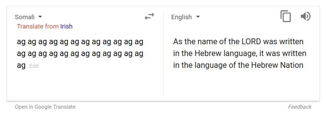
So is Machine Translation solved?
• Nope!
• Uninterpretable systems do strange things
• (But I think this problem has been fixed in Google Translate by 2021?)

 Picture source: https://www.vice.com/en_uk/article/j5npeg/why-is-google-translate-spitting-out-sinister-religious-prophecies
 Explanation: https://www.skynettoday.com/briefs/google-nmt-prophecies
55

NMT research continues
NMT is a flagship task for NLP Deep Learning

• NMT research has pioneered many of the recent innovations of NLP Deep Learning

• In 2021: NMT research continues to thrive
 • Researchers have found many, many improvements to the “vanilla” seq2seq NMT
 system we’ve just presented

 • But we’ll present in a minute one improvement so integral that it is the new vanilla…

 ATTENTION
56

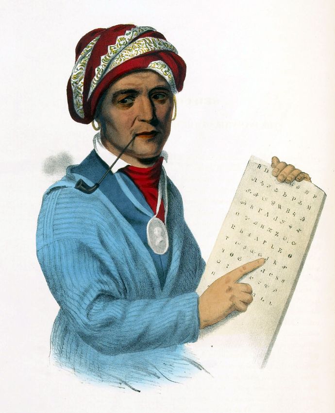
Assignment 4: Cherokee-English machine translation!
• Cherokee is an endangered Native American language – about 2000 fluent speakers
• Extremely low resource: About 20k parallel sentences available, most from the bible
• ᎪᎯᎩᏴ ᏥᎨᏒᎢ ᎦᎵᏉᎩ ᎢᏯᏂᎢ ᎠᏂᏧᏣ. ᏂᎪᎯᎸᎢ ᏗᎦᎳᏫᎢᏍᏗᎢ ᏩᏂᏯᎡᎢ
 ᏓᎾᏁᎶᎲᏍᎬᎢ ᏅᏯ ᎪᏢᏔᏅᎢ ᎦᏆᏗ ᎠᏂᏐᏆᎴᎵᏙᎲᎢ ᎠᎴ ᎤᏓᏍᏈᏗ ᎦᎾᏍᏗ ᎠᏅᏗᏍᎨᎢ
 ᎠᏅᏂᎲᎢ.
 Long ago were seven boys who used to spend all their time down by the townhouse
 playing games, rolling a stone wheel along the ground, sliding and striking it with a stick
• Writing system is a syllabary of symbols for each CV unit (85 letters)
• Many thanks to Shiyue Zhang, Benjamin Frey, and Mohit Bansal
 from UNC Chapel Hill for the resources for this assignment!

• Cherokee is not available on Google Translate! 

57

Cherokee
• Cherokee originally lived in western North Carolina and eastern Tennessee
• Most speakers now in Oklahoma, following the Trail of Tears; some in NC
• Writing system Invented by Sequoyah around 1820 – someone who
 was previously illiterate
 • Very effective: In the following decades Cherokee literacy was higher
 than for white people in the southeastern United States

• https://www.cherokee.org

58

Section 3: Attention

59

Sequence-to-sequence: the bottleneck problem
 Encoding of the
 source sentence.
 Target sentence (output)

 he hit me with a pie 
 Encoder RNN

 Decoder RNN
 il a m’ entarté he hit me with a pie

 Source sentence (input)

 Problems with this architecture?

60

Sequence-to-sequence: the bottleneck problem
 Encoding of the
 source sentence.
 This needs to capture all Target sentence (output)
 information about the
 source sentence. he hit me with a pie 
 Information bottleneck!
 Encoder RNN

 Decoder RNN
 il a m’ entarté he hit me with a pie

 Source sentence (input)

61

Attention
• Attention provides a solution to the bottleneck problem.

• Core idea: on each step of the decoder, use direct connection to the encoder to focus
 on a particular part of the source sequence

• First, we will show via diagram (no equations), then we will show with equations

62

Sequence-to-sequence with attention

 dot product
 Attention
 scores

 Decoder RNN
 Encoder
 RNN

 il a m’ entarté 

63
 Source sentence (input)

Sequence-to-sequence with attention

 dot product
 Attention
 scores

 Decoder RNN
 Encoder
 RNN

 il a m’ entarté 

64
 Source sentence (input)

Sequence-to-sequence with attention

 dot product
 Attention
 scores

 Decoder RNN
 Encoder
 RNN

 il a m’ entarté 

65
 Source sentence (input)

Sequence-to-sequence with attention

 dot product
 Attention
 scores

 Decoder RNN
 Encoder
 RNN

 il a m’ entarté 

66
 Source sentence (input)

Sequence-to-sequence with attention

 On this decoder timestep, we’re
 scores distribution mostly focusing on the first
 encoder hidden state (”he”)
 Attention Attention

 Take softmax to turn the scores
 into a probability distribution

 Decoder RNN
 Encoder
 RNN

 il a m’ entarté 

67
 Source sentence (input)

Sequence-to-sequence with attention
 Attention Use the attention distribution to take a
 output weighted sum of the encoder hidden
 scores distribution states.
 Attention Attention

 The attention output mostly contains
 information from the hidden states that
 received high attention.

 Decoder RNN
 Encoder
 RNN

 il a m’ entarté 

68
 Source sentence (input)

Sequence-to-sequence with attention
 Attention he
 output
 Concatenate attention output
 scores distribution
 !! with decoder hidden state, then
 Attention Attention

 use to compute !1 as before

 Decoder RNN
 Encoder
 RNN

 il a m’ entarté 

69
 Source sentence (input)

Sequence-to-sequence with attention
 Attention hit
 output
 scores distribution
 !"
 Attention Attention

 Decoder RNN
 Encoder
 RNN

 Sometimes we take the
 attention output from the
 previous step, and also
 feed it into the decoder
 il a m’ entarté he (along with the usual
 decoder input). We do
 this in Assignment 4.
70
 Source sentence (input)

Sequence-to-sequence with attention
 Attention me
 output
 scores distribution
 !#
 Attention Attention

 Decoder RNN
 Encoder
 RNN

 il a m’ entarté he hit

71
 Source sentence (input)

Sequence-to-sequence with attention
 Attention with
 output
 scores distribution !$
 Attention Attention

 Decoder RNN
 Encoder
 RNN

 il a m’ entarté he hit me

72
 Source sentence (input)

Sequence-to-sequence with attention
 Attention a
 output
 scores distribution !%
 Attention Attention

 Decoder RNN
 Encoder
 RNN

 il a m’ entarté he hit me with

73
 Source sentence (input)

Sequence-to-sequence with attention
 Attention pie
 output
 scores distribution !&
 Attention Attention

 Decoder RNN
 Encoder
 RNN

 il a m’ entarté he hit me with a

74
 Source sentence (input)

Attention: in equations
• We have encoder hidden states
• On timestep t, we have decoder hidden state
• We get the attention scores for this step:

• We take softmax to get the attention distribution for this step (this is a probability distribution and
 sums to 1)

• We use to take a weighted sum of the encoder hidden states to get the
 attention output

• Finally we concatenate the attention output with the decoder hidden
 state and proceed as in the non-attention seq2seq model

75

Attention is great
• Attention significantly improves NMT performance
 • It’s very useful to allow decoder to focus on certain parts of the source
• Attention solves the bottleneck problem
 • Attention allows decoder to look directly at source; bypass bottleneck
• Attention helps with vanishing gradient problem
 • Provides shortcut to faraway states
• Attention provides some interpretability
 • By inspecting attention distribution, we can see

 with
 me

 pie
 he
 hit

 a
 what the decoder was focusing on il

 • We get (soft) alignment for free! a

 • This is cool because we never explicitly trained m’

 an alignment system entarté

 • The network just learned alignment by itself

76

Attention is a general Deep Learning technique
• We’ve seen that attention is a great way to improve the sequence-to-sequence model
 for Machine Translation.
• However: You can use attention in many architectures
 (not just seq2seq) and many tasks (not just MT)

• More general definition of attention:
 • Given a set of vector values, and a vector query, attention is a technique to compute
 a weighted sum of the values, dependent on the query.

• We sometimes say that the query attends to the values.
• For example, in the seq2seq + attention model, each decoder hidden state (query)
 attends to all the encoder hidden states (values).

77

Attention is a general Deep Learning technique
 More general definition of attention:
 Given a set of vector values, and a vector query, attention is a
 technique to compute a weighted sum of the values, dependent on
 the query.

 Intuition:
 • The weighted sum is a selective summary of the information
 contained in the values, where the query determines which
 values to focus on.
 • Attention is a way to obtain a fixed-size representation of an
 arbitrary set of representations (the values), dependent on
 some other representation (the query).

78

There are several attention variants
• We have some values and a query

• Attention always involves: There are
 multiple ways
 1. Computing the attention scores
 to do this
 2. Taking softmax to get attention distribution ⍺:

 3. Using attention distribution to take weighted sum of values:

 thus obtaining the attention output a (sometimes called the context vector)

79

You’ll think about the relative
Attention variants advantages/disadvantages of these in Assignment 4!

There are several ways you can compute from
and :

• Basic dot-product attention:
 • Note: this assumes
 • This is the version we saw earlier

• Multiplicative attention:
 • Where is a weight matrix

• Additive attention:
 • Where are weight matrices and
 is a weight vector.
 • d3 (the attention dimensionality) is a hyperparameter
 More information: “Deep Learning for NLP Best Practices”, Ruder, 2017. http://ruder.io/deep-learning-nlp-best-practices/index.html#attention
 “Massive Exploration of Neural Machine Translation Architectures”, Britz et al, 2017, https://arxiv.org/pdf/1703.03906.pdf
80

Summary of today’s lecture
 • We learned some history of Machine Translation (MT)

 • Since 2014, Neural MT rapidly
 replaced intricate Statistical MT

 • Sequence-to-sequence is the
 architecture for NMT (uses 2 models: encoder and decoder)

 • Attention is a way to focus on
 particular parts of the input
 • Improves sequence-to-sequence a lot!
81