Comparison of two community noise models applied to a NASA urban air mobility concept vehicle
←
→
Page content transcription
If your browser does not render page correctly, please read the page content below
Comparison of two community noise models applied to a NASA
urban air mobility concept vehicle
Stephen A. Rizzi 1
Aeroacoustics Branch, NASA Langley Research Center
Hampton, VA 23681-2199, USA

Juliet A. Page 2
Volpe National Transportation Systems Center, 55 Broadway
Cambridge, MA 02142-1093, USA

Rui Cheng 3
National Institute of Aerospace, 100 Exploration Way
Hampton, VA 23666-6266, USA

                                         ABSTRACT
Predictions of community noise exposure from a NASA urban air mobility (UAM) concept
vehicle have been conducted for representative operations using the FAA Aviation
Environmental Design Tool (AEDT) in order to demonstrate modeling tool interoperability
and assess applicability, capabilities and limitations of integrated noise modeling tools. To
both quantify limitations and highlight other capabilities, a comparative analysis is
performed using a time-domain simulation method, in particular, using the Volpe Advanced
Acoustic Model (AAM). Using the same source noise model, the 3D directivity of a UAM
concept vehicle is predicted in terms of aeroacoustic pressure time histories at a sphere of
observer positions near the vehicle. In addition to distilling those data to a set of noise-power-
distance data for input to AEDT, the data are processed preserving spectral directivity, into
one-third and one-twelfth octave bands for input to AAM. Results from AEDT and AAM
modeling are provided for a variety of metrics to demonstrate the effect that source noise
directivity and propagation modeling fidelity have on predicted results at receptors over a
study area.
1.   INTRODUCTION
   A comparative analysis was conducted with the FAA’s Aviation Environmental Design Tool
(AEDT) [1] and the Volpe Advanced Acoustic Model (AAM) [2] for the purposes of assessing
modeling applicability, capabilities and limitations, and identifying potential future modeling

1
  stephen.a.rizzi@nasa.gov
2
  juliet.page@dot.gov
3
  rui.cheng@nasa.gov
improvements. AEDT is an integrated model developed for assessing cumulative noise impacts
from aviation noise sources. It includes vehicle source directivity adequate for assessing fixed-
wing and conventional rotary-wing community noise, but has limited ability for considering
complex advanced air mobility configurations. A set of noise spheres with full three-dimensional
spectral directivity in one-third octave band and one-twelfth octave bands was modeled for a
NASA quadrotor reference vehicle. These noise spheres were used to model a selected flight
operation in AAM to benchmark A-weighted metric results on ground contours and points of
interest for the purposes of comparison with AEDT. Derivative omnidirectional and axisymmetric
noise spheres were also developed to evaluate the impact of limited directivity assumptions. Some
advanced AAM analyses using acoustic visualization, narrow band analysis and calculation of
time varying loudness metrics were conducted to aid in interpreting acoustic results.
2.   CONCEPT VEHICLES, TRAJECTORIES, AND OPERATING STATES
2.1. Vehicle Descriptions
     Noise from the quadrotor reference vehicle developed under the NASA Revolutionary
Vertical Lift Technology (RVLT) Project was investigated in this paper, see Figure 1. The vehicle
was sized for a 1200 lb. payload (up to six passengers) executing a representative mission profile
[3]. The quadrotor was an all-electric variant, with three-bladed rotors, gross weight of 6469 lb.,
and maximum airspeed Vmax of 109 knots true airspeed (KTAS). Additional details on this
configuration can be found in Ref. [4].
2.2. Trajectory Data
     Trajectory data were generated using a mission planner algorithm developed by NASA for
UAM operations research [5]. The route data are the same as those used in the X2 engineering
evaluation conducted by the NASA Air Traffic Management – Exploration (ATM-X) Project,
UAM subproject. The X2 evaluation consisted of sixteen routes in the Dallas-Ft. Worth, TX, area.
The maximum airspeed was limited to 85% of Vmax.
2.3. Determination of Operating States
     The trajectory data were reduced to determine aircraft operational states for which noise
estimates are needed, see Section 3. In this paper, the aircraft operational states are defined by
pairs of airspeed (knots) and climb angle (deg.). It was considered impractical to generate noise
estimates based on 1 Hz trajectory data for each of the sixteen routes. A condensation scheme was
developed to select operational states based on the number of occurrences (counts) over sixteen
routes [6]. This resulted in 42 unique operating states, as shown in Figure 2. A unique numerical
identifier, e.g., 101, 102, etc., was used to identify the particular operating state.
3.   SOURCE NOISE DATA GENERATION
     This section describes the process for generating user-defined source noise sphere data
through analysis. The process involves two steps; the first step determines the trimmed condition
at each operating state and the second step performs the acoustic analysis. A summary of each
step follows. The overall process, depicted in Figure 3, is a subset of that used to generate noise-
power-distance (NPD) data for input to AEDT [6].
3.1. Vehicle Trim
     Given the vehicle configuration and prescribed operating state, the vehicle is “trimmed” in an
iterative fashion using a comprehensive analysis code. In the trimmed condition, the control
surface configuration of the vehicle corresponds to the desired flight condition. For this work, the
Comprehensive Analytical Model of Rotorcraft Aerodynamics and Dynamics (CAMRAD II) [7]
was used to trim the vehicle.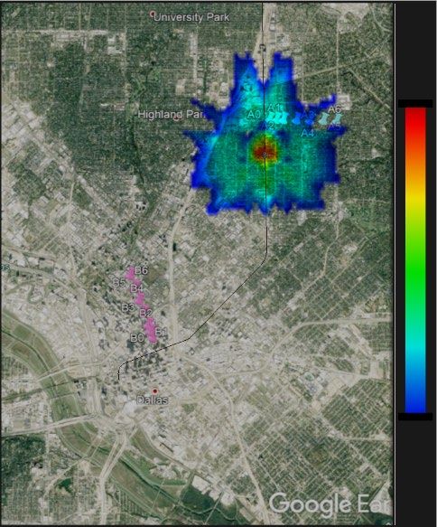
Figure 1: NASA RVLT quadrotor reference            Figure 2: Operating states for the quadrotor
 vehicle configuration considered in this study.                 reference vehicle.

          Figure 3: NASA process for generating source noise data for input to AAM.
     The rotors on the quadrotor vehicle operate at a constant RPM with a 20 Hz blade passage
frequency (BPF) and utilize collective pitch control. The trim targets are the six degrees-of-
freedom (Fx, Fy, Fz, Mx, My, and Mz), and trim variables include four collective control
combinations of rotor pairs, plus vehicle pitch and roll. The same trim mode was used at all speeds.
3.2. Source Noise Spheres
     The resulting blade loadings and motion from the trim operation serve as input to a system
noise prediction. In this work, the ANOPP2 Aeroacoustic ROtor Noise (AARON) tool, a part of
the NASA 2nd generation Aircraft Noise Prediction Program (ANOPP2) [8], was used for the
system noise prediction. The acoustics solver uses Farassat’s Formulation F1A [9] to compute the
periodic loading and thickness noise components under a quasistatic operating condition at a set
of observers at a fixed radius from the aircraft center of gravity. The set of observers constitutes
the source noise sphere and the two noise components included constitute the so-called first
generation (Gen 1.2) database. Although only the lower hemisphere of observers (below the
vehicle) was computed in this work, the more general sphere usage is retained. Each source noise
sphere (one for each operating state) is exported as one-third and one-twelfth octave band data to
a NetCDF file for input to AAM. Per AAM compact source modeling requirements, noise spheres
are referenced to a finite radius. Spectral data on the noise sphere were provided on a spherical
coordinate system mesh with 10o spacing. The polar angle, θ, ranges from 0° at the nose to 180°
at the tail, while the azimuth angle, φ, ranges from -90° on the port (left) side to +90° on the
starboard (right) side.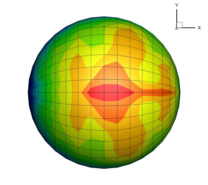
Sample source noise data in the form of one-third octave band sound pressure levels (SPL)
are shown in Figure 4 for a low speed ascent condition (10 knot airspeed and 85° climb angle) and
high speed descent condition (60 knot airspeed and -5° climb angle), and in the left-hand side of
Figure 5 for a high speed cruise condition (90 knot airspeed and 0° climb angle). The data
represent the 20 Hz one-third octave band incorporating the BPF. The higher levels for the high
speed descent condition are due to the presence of blade-vortex interaction noise, as evidenced by
blade loading data (not shown). The source data may be highly directional, as also evidenced by
the overall SPL on the right-hand side of Figure 5. In contrast, the NPD used in the companion
AEDT analyses are derived from source data along the centerline (0° azimuth), with an assumed
90° dipole directivity used in the noise fraction adjustment for fixed-wing aircraft. Consequently,
AAM and AEDT predictions are expected to best agree under the flight track, and differ at lateral
locations due, in part, to differences in source spectral directivity.

Figure 4: Source noise data for low speed ascent (left) and high speed descent (right) conditions
            in the 20 Hz one-third octave band. Nose is in the positive x-direction.

 Figure 5: Source noise data for high speed cruise condition in the 20 Hz one-third octave band
     (left) and the overall sound pressure level (right). Nose is in the positive x-direction.
    The NPD values for A-weighted sound exposure level (SELA) and maximum A-weighted
sound pressure level (LmaxA) used in the AEDT analyses were computed using the 3D noise
spheres, see companion paper [6] for details. Azimuthal source directivity was not directly
accounted for because the AEDT analyses were performed using a fixed-point flight profile
method for fixed-wing propeller aircraft. Consequently, the NPD values reflected only the polar
spectral directivity along the 0° azimuth, versus a better representation of azimuthal directivity that
could be achieved using AEDT helicopter modes or the full 3D directivity in AAM using the
ANOPP2 sphere.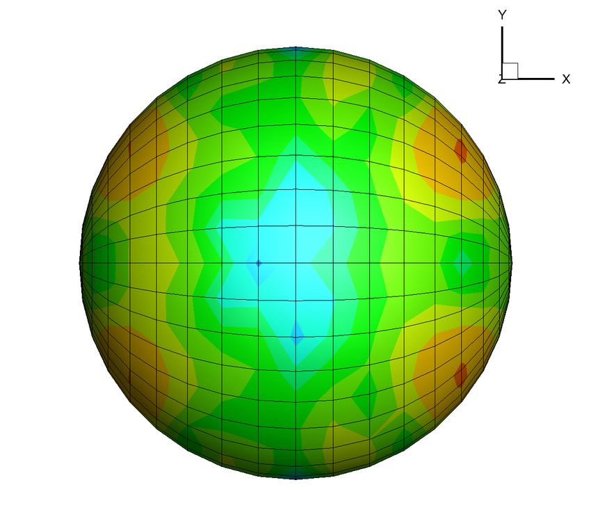
4.   AAM MODELING
4.1. Trajectory Data
     AAM input trajectory data were developed from the combination of AEDT track and profile
point data specified in the companion paper [6]. Using the NCSPEC option for AAM input, each
trajectory point consisted of x and y coordinates in Universal Transverse Mercator (UTM)
coordinates, the altitude, airspeed, operating state identifier (via AAM keyword NCSPEC), and
other parameters related to the attitude of the aircraft. The latter were set to model level flight as
the aircraft attitude was already reflected in the source noise sphere data. In AAM, additional
simulation time steps were interpolated from the input trajectory in order to achieve at least 0.5 sec
time spacing. In using the NCSPEC option, AAM utilizes a constant noise source between
simulation points; however, AAM will interpolate on speed when developing the simulation
trajectory. To limit that, a ‘guard’ track point, having the same operating state identifier and speed
as the previous track point, is inserted just prior to the next input trajectory point. In doing so,
interpolation of speed is limited to a short (12 ft.) transition segment. To the maximum extent
possible, this replicated the conditions under which the AEDT analyses were performed using a
fixed-point flight profile methodology outlined in the companion paper.
4.2. Calibration of Noise Spheres for AAM
      A calibration process is utilized in order to account for differences in the AAM and AEDT
propagation models. A reference trajectory was chosen based on the most prevalent cruising
condition, namely 90 knots level flight at 1000 ft. altitude. An idealized trajectory at the reference
condition was developed in AEDT and the undertrack centerline LmaxA was calculated using the
NPD data [6]. The corresponding noise sphere was analyzed in AAM and a spectrally uniform
calibration factor was applied over the entire sphere so that LmaxA predictions matched between
AAM and AEDT. The resulting calibration factors (see below) were found to be very small.
AEDT results are reported for grid receptors at 4 ft. above ground level (AGL) and a corresponding
4 ft. AGL height was used for AAM Points of Interest (POIs) with a matched slant range (1000 ft.)
between the source and receiver at the point of closest approach (directly overhead).
      Three different noise spheres were generated using derivative information from the analysis
described in the companion paper [6] and calibrated using the reference trajectory. These spheres
include:
         • Omnidirectional – undertrack spectra at the point of LmaxA repeated in all directions
             (Figure 6, Calibration: +0.33 dB)
         • Axisymmetric – undertrack polar spectral directivity repeated at all azimuthal angles
             (Figure 7, Calibration: +0.21 dB)
         • Full 3D – based on the ANOPP2-based modeling described in Section 3.2 (as shown
             uncalibrated on the right-hand side of Figure 5, Calibration: +0.21 dB)
4.3. Comparison of AEDT with AAM Omnidirectional Sphere Results at Lateral POIs
     The reference case described in Section 4.2 was modeled in AEDT and AAM. Results (SELA
and LmaxA) were predicted at a series of receptors undertrack and at lateral distances of 500,
1000, 2000, 3000, 4000 and 5000 ft. and compared using the calibrated omnidirectional,
axisymmetric and 3D spheres. Table 1 lists the POIs and the corresponding sphere angles.
Y
Sound Pressure Level (dB, rel. 20 µ Pa)   80

                                                                                                                                             Z        X
                                          70

                                          60                                                                                                     SPL (dB)
                                                                                                                                                     82
                                                                                                                                                     80
                                                                                                                                                     78
                                          50                                                                                                         76
                                                                                                                                                     74
                                                                                                                                                     72
                                                                                                                                                     70
                                          40                                                                                                         68
                                                                                                                                                     66
                                                                                                                                                     64
                                                                                                                                                     62
                                          30

                                          20

                                          10 1
                                           10                102             103               104
                                                 One-Third Octave Band Center Frequency (Hz)
   Figure 6: Quadcopter spectrum for 90 kt level                                                     Figure 7: Axisymmetric sphere (unweighted),
   flight for omnidirectional sphere (calibrated).                                                    90 kt level flight (calibrated). Nose to right.
                                      Table 1: AAM sphere geometric information at points corresponding to LmaxA at the POIs.
                                                                                                  Geometry for LmaxA
                                               Receiver            Lateral Dist (ft.)          Phi (deg)        Theta (deg)       Slant Range (ft.)
                                                  1                       0                        0                79                  1019
                                                  2                      500                     -27                70                  1194
                                                  3                     1000                     -45                61                  1624
                                                  4                     2000                     -63                50                  2909
                                                  5                     3000                     -72                50                  4107
                                                  6                     4000                     -76                80                  4186
                                                  7                     5000                     -79                60                  5878
AAM Omnidirectional Sphere
     Since the sphere calibration was conducted for LmaxA for a 1000 ft. slant range, directly
undertrack, these predictions are identical (Figure 8, AEDT: red, AAM: black) at that range. The
SELA values differ by 1.7 dB and this is attributable to polar spectral directivity that accumulates
in the SELA calculation. The NPD generation analysis was based on a slice of the 3D sphere along
the centerline (right-hand side of Figure 5) which exhibits considerable variation from nose to tail,
whereas the AAM analysis utilizes a single spectrum in all directions on the sphere (Figure 6).
The SELA metric is computed from the full time history (within 10 dB of the maximum) while
the LmaxA metric is only matched at the peak of the time history.
Comparison of AEDT with AAM Axisymmetric Sphere Results at Lateral POIs
     For the case where AEDT lateral results are compared with the AAM axisymmetric results
(Figure 9), the undertrack levels at 1000 ft. for both SELA and LmaxA are identical due to the
consistency in the polar directivity for the two models. For other lateral locations, slight
differences are noted and are due to different propagation models used in AAM and AEDT. The
AEDT analysis modeled the vehicle as a propeller aircraft, which does not include azimuthal
source directivity, and is functionally equivalent to the AAM axisymmetric sphere. Note that
AAM includes a more sophisticated ground effects model than AEDT that considers direct and
reflected rays and can exhibit significant ‘dips’ in the received sound spectrum.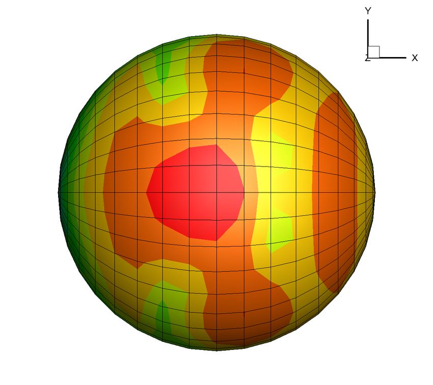
80                                                                                               80
                                                                    AEDT, SELA                                                                                          AEDT, SELA
                            75                                      AEDT, LmaxA                                              75                                         AEDT, LmaxA
                                                                    AAM, SELA                                                                                           AAM, SELA
                            70                                      AAM, LmaxA                                               70                                         AAM, LmaxA
 Level (dBA, rel: 20 µPa)

                                                                                   Level (dBA, rel: 20 µPa)
                            65                                                                                               65

                            60                                                                                               60

                            55                                                                                               55

                            50                                                                                               50

                            45                                                                                               45

                            40                                                                                               40

                            35                                                                                               35

                            30                                                                                               30
                                 0   1000      2000      3000       4000    5000                                                  0   1000      2000        3000        4000    5000
                                            Lateral Distance (ft)                                                                            Lateral Distance (ft)
Figure 8: Metric comparison AEDT vs. AAM                                              Figure 9: Metric comparison AEDT vs.
   (omnidirectional sphere) at lateral POIs.                                       AAM (axisymmetric sphere) at lateral POIs.
Comparison of AEDT with AAM 3D Sphere Results at Lateral POIs
    Significant differences in the metric prediction at lateral positions are evident between AAM
and AEDT when using the 3D spheres (Figure 10). This is primarily due to differences in
azimuthal directivity and provides an example of potential differences between simplified source
modeling for fixed-wing aircraft in AEDT and 3D sources in AAM.
Examination of AAM Time Histories at Lateral POIs
     The A-weighted sound pressure level time history is provided in Figures 11 and 12 for the
undertrack and 3000 ft. lateral POIs, respectively. Figure 11 shows a comparison of the time
history at the undertrack POI between the three spheres, where the differences in polar directivity
are evident. The axisymmetric and 3D sphere results align perfectly for the entire time history as
expected, since the axisymmetric sphere was developed from the 3D centerline polar spectral
directivity.
                            80                                                                                               65
                                                                    AEDT, SELA
                                                                                   Sound Pressure Level (dBA, rel: 20 µPa)

                            75                                      AEDT, LmaxA
                                                                    AAM, SELA                                                60
                            70                                      AAM, LmaxA
 Level (dBA, rel: 20 µPa)

                            65                                                                                               55

                            60
                                                                                                                             50
                            55
                                                                                                                             45
                            50

                            45                                                                                               40
                                                                                                                                                      Omnidirectional
                            40                                                                                                                        Axisymmetric
                                                                                                                             35                       3D
                            35

                            30                                                                                               30
                                 0   1000      2000      3000       4000    5000                                              700     710       720          730        740      750
                                            Lateral Distance (ft)                                                                                Time (sec)
                Figure 10: Metric comparison AEDT vs.                              Figure 11: AAM undertrack sound pressure
                   AAM (3D sphere) at lateral POIs.                                level time histories for 3 calibrated spheres.
     At the 3000 ft. lateral POI location (Figure 12), one can see significant amplitude and shape
differences throughout the time history. Differences in polar directivity for the 3D and
axisymmetric spheres results in LmaxA occurring at different times. The differences in the LmaxA
levels are also reflected in Figure 10 at the 3000 ft. lateral location. The unsteadiness in the time
history traces in Figure 11 and Figure 12 is due to ground effects for the 4 ft. receiver height. This
behavior is also evident in the selected time history bands for the 3D sphere at the undertrack
location, as shown in Figure 13.
                                                                                                80                              20 Hz
                                                                                                                                63 Hz

                                                      Sound Pressure Level (dBA, rel: 20 µPa)
                                                                                                                                100 Hz
                                                                                                                                500 Hz
                                                                                                                                1 kHz
                                                                                                60                              2 kHz

                                                                                                40

                                                                                                20

                                                                                                 0
                                                                                                 290   310      330       350      370
                                                                                                             Time (sec)

Figure 12: AAM sideline sound pressure level         Figure 13: AAM undertrack one-third octave
    time histories for 3 calibrated spheres.          band sound pressure level time histories for
                                                                calibrated 3D sphere.
5.   SAMPLE RESULTS
5.1. AAM and AEDT Analysis for a Selected Operation
     One of sixteen routes, KCAT-KDT4 [6], was selected for an in-depth analysis using AAM in
order to illustrate and compare analyses results and provide visual insight. The spheres used in
this section were calibrated using the process described in Section 4.2. The same calibration factor,
based on the 90 kts level flight condition, was used for each of the 42 quadcopter spheres prior to
AAM analysis. This was done to reduce complexity and scope. However, one could also calibrate
each of the other flight condition spheres individually using a similar process.
5.2. Metric Comparison at Points of Interest near Takeoff and Landing Sites
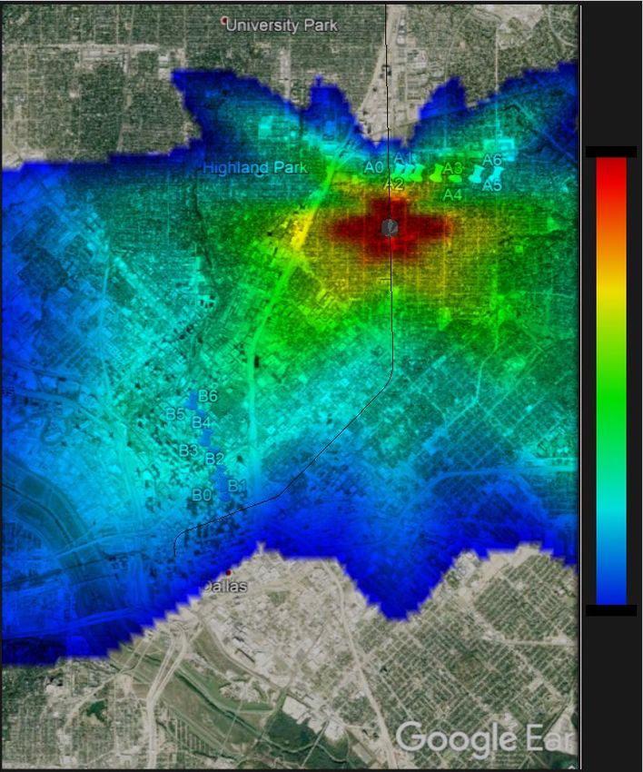
     Four series of points were identified for comparison of metrics between AEDT and AAM, see
Figure 14. Each includes one undertrack location and six lateral locations up to 5000 ft. sideline
ground distance. Figure 15 shows the ‘Cruz’ POIs areas in the takeoff and landing regions. The
AEDT overpredictions, compared with the AAM simulations using the full 3D source directivity,
are consistent with those in the reference case described in Section 4.3.
5.3. Contour Comparison
     AEDT and AAM contours of LmaxA and SELA are provided in Figures 16 and 17,
respectively. One can see that the LmaxA contours from AEDT in the vicinity of vertiports are
nearly circular as the source is essentially a monopole. In contrast, the LmaxA contours from
AAM reflect the more complex directivity character. Likewise, the SELA contours from AEDT
(Figure 17) reflect the simplified 90 deg. dipole used in the AEDT noise fraction calculation for
fixed-wing aircraft, whereas those from AAM exhibit the true 3D directivity with lower levels at
lateral locations. Both sets of results compare favorably under the track, but increasingly differ
away from the track, in part due to the previously noted lateral attenuation differences between
AEDT and AAM. The abrupt transitions between spheres are seen in the AAM results since the
NCSPEC keyword does not allow interpolation between different spheres.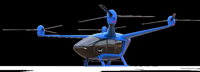
(a)                                               (b)
               Figure 14: Flight track and points of interest near the KCAT-KDT4
          takeoff region (a) and landing region (b) with 5000 ft. grid spacing indicated.

                                                                                                 75
                                                                                                                      KDT4 (Cruz)
                                                       Sound Pressure Level (dBA, rel: 20 µPa)
                                                                                                 70

                                                                                                 65

                                                                                                 60

                                                                                                 55

                                                                                                 50

                                                                                                 45

                                                                                                 40
                                                                                                                 AEDT, SELA
                                                                                                 35              AEDT, LmaxA
                                                                                                                 AAM, SEL
                                                                                                 30              AAM, LmaxA

                                                                                                 25
                                                                                                      0   1000        2000      3000       4000   5000
                                                                                                                   Lateral Distance (ft)

  Figure 15: Metric comparisons for ‘Cruz’ POIs near takeoff (left) and landing (right) regions.
5.4. Acoustic Simulation Visualization using AAM
     AAM can be used to create animations in a variety of metrics and individual one-third or one-
twelfth octave bands, in order to visualize acoustic influences of vehicle directivity and transition
segments, and to assess impacts on the ground. Acoustic visualization is also helpful to understand
specific features seen in spectral time histories. The instantaneous LmaxA footprint illustrated in
Figure 18 (a) is from a point where the vehicle passes over the takeoff cruise points of interest near
KCAT. The swirling is due to differences in arrival times for various portions of the directivity
pattern emitted at different heading angles. Figure 18 (b) illustrates the 20 Hz one-third octave
band later in the cruise portion of the trajectory (shortly after the vehicle has passed over the
approach POI). Note the clear indication of the lobes in the directivity pattern, including those aft
of the vehicle. When viewing the acoustic animations (available for download [10, 11]),
transitions between operating modes are apparent, and can aid in the design of operational
procedures as well as in the understanding of how 3D spectral directivity data affect auralized
sounds, such as those from the NASA Auralization Framework [12].
KDT4
11935000
35
60
55
45
KCAT
45
12045000 11930000 40
55
50 11925000
60
12040000 LmaxA (dBA)
40
60
65 LmaxA (dBA)
30
80
50
35
35
50
45 65 75
11920000 70
45
12035000 60 55
45
Y UTM (ft)
30
65
Y UTM (ft)
55
45 55
60
60
50
45
40
45 11915000 55
12030000
60
40 50
55
45
50
50 35
70
40
50
30 11910000 65 40
12025000
60
25 75 65 35
35
75
35
50
60
20 70 30
60 5
55
15 25
45
11905000
45
5
12020000
45
55 20
30
55
40
50 45
60 11900000
12015000
2290000 2300000 2310000 2320000
X UTM (ft)
11895000
2310000 2320000 2330000
X UTM (ft)
Figure 16: Comparison of AEDT (lines) and AAM (color fill) LmaxA contours in the
takeoff (left) and landing (right) areas over the calculation region identified in Figure 14.
KDT4
11935000
70
55
KCAT 11930000
12045000
50
55
35 5 45
550
12040000 40 11925000 SELA (dBA)
SELA (dBA)
65
70
85
60
65
80
60
70
60
45
65 11920000 75
12035000
65
Y UTM (ft)
70
Y UTM (ft)
60
70
55 65
55
11915000
70
60
60
50
50
12030000
65
50
55
75 55
45
55
55
40 50
35 11910000 45
60
12025000 80 40
30
65
85
60
70
70
65
65
25 35
30
45
11905000
12020000
60
70
70
60
11900000
55
65
12015000
50
55
50
2290000 2300000 2310000 2320000
X UTM (ft)
11895000
2310000 2320000 2330000
X UTM (ft)
Figure 17: Comparison of AEDT (lines) and AAM (color fill) SELA contours in the
takeoff (left) and landing (right) areas over the calculation region identified in Figure 14.
5.5. Advanced Analyses using AAM
Additional capabilities have been recently added to AAM to facilitate in-depth analysis of
advanced air mobility vehicle operations; including computation of time varying loudness (TVL)
metrics in the presence of background noise spectra, instantaneous loudness (sone), short term
(ST) and long term (LT) loudness (sone), d' (d prime), and long term loudness level (phon) from
one-third or one-twelfth octave bands [13, 14]. In this example, the same KCAT-KDT4 operation
was examined using calibrated one-twelfth octave band noise spheres. Empirical ambient noise
spectra [15] obtained in the Dallas area for the morning rush hour and in the quiet nighttime were
used to assess TVL for the POIs under consideration. An example TVL time history for a point at
500 ft. sideline to the cruise-approach transition in Figure 19 illustrates multiple peaks near the
point of closest approach. In this demonstration, the values of d' indicate that the vehicle would
be audible during the nighttime, but not in the daytime. Examination of the footprint in Figure 19
suggests that the directivity lobes are responsible for these details. Although the quadrotor vehiclenoise spheres include only loading and thickness noise and the trajectories are simplified and not
optimized, these advanced analysis capabilities can aid the vehicle and operational route designer.
(a) (b)
Figure 18: AAM temporally interpolated instantaneous ground receiver levels using
3D calibrated spheres at two locations for the KCAT-KDT4 operation.
41.2 ST Loudness (AM Rush) 16 20
Loudness (sone) [Nighttime Background]
Loudness (sone) [AM Rush Background]
LT Loudness (AM Rush)
DPRIME (AM Rush)
ST Loudness (Night)
LT Loudness (Night)
DPRIME (Night) 15
41 10
14
13
DPRIME
40.8 0
12
11
40.6 -10
10
40.4 9 -20
40 60 80 100 120
Time (sec)
Figure 19: Computed TVL metrics at a 500 ft. sideline POI near the cruise-approach transition
(left) and the 100 Hz footprint for a time just after the vehicle has passed over this POI (right).
6. CONCLUDING REMARKS
Comparative analyses between AEDT and AAM suggest that 3D spectral directivity can be
an important feature to capture, particularly at lateral locations. However, these observations are
based on data that do not include broadband noise, which may dominate at higher frequencies and
result in a more uniform directivity. Subsequent noise generation data, containing broadband self
noise, may be used to assess that possibility. Acoustic visualization tools can be used to assess
impacts of 3D spectral directivity and the influence of operational procedure design. Time varying
loudness metrics can be assessed against differing backgrounds at points of interest or over a grid.
Future plans include an evaluation of the helicopter modeling capability within AEDT, which will
allow right-center-left directivity to be incorporated in the analyses, and demonstrating the
feasibility of developing visualization and auralization from a common analysis. Long term AAMdevelopment plans include the development of automated sphere selection and interpolation
procedures for advanced air vehicles.
7. ACKNOWLEDGMENTS
This work was partially supported by the NASA Aeronautics Research Mission Directorate,
Revolutionary Vertical Lift Technology Project. The authors wish to acknowledge Doug Boyd
(NASA Langley) for the AARON tool development and assistance in generating source noise
spheres.
8. REFERENCES
1. "Aviation Environmental Design Tool (AEDT) technical manual, Version 3c," U.S.
Department of Transportation, Volpe National Transportation Systems Center, Cambridge,
MA, DOT-VNTSC-FAA-20-05, 2020.
2. "Advanced Acoustic Model (AAM), Technical Reference and User's Guide," U.S.
Department of Transportation, Volpe National Transportation Systems Center, Cambridge,
MA, DOT-VNTSC-20-05, 2020.
3. Patterson, M.D., Antcliff, K.R., and Kohlman, L.W., "A proposed approach to studying
urban air mobility missions including an initial exploration of mission requirements," AHS
International 74th Annual Forum and Technology Display, Phoenix, AZ, 2018.
4. Silva, C., Johnson, W.R., Solis, E., Patterson, M.D., and Antcliff, K.R., "VTOL urban air
mobility concept vehicles for technology development," AIAA AVIATION Forum, AIAA-
2018-3847, Atlanta, GA, 2018.
5. Guerreiro, N.M., Butler, R.W., Maddalon, J.M., and Hagen, G.E., "Mission planner
algorithm for urban air mobility – Initial performance characterization," AIAA AVIATION
Forum, AIAA-2019-3626, Dallas, TX, 2019.
6. Rizzi, S.A. and Rafaelof, M., "Community noise assessment of urban air mobility vehicle
operations using the FAA Aviation Environmental Design Tool," InterNoise 2021, Virtual
Meeting, 2021.
7. Johnson, W.R., "Rotorcraft aerodynamic models for a comprehensive analysis," AHS
International 54th Annual Forum, Washington, DC, 1998.
8. Lopes, L.V. and Burley, C.L., "ANOPP2 User's Manual: Version 1.2," NASA TM-2016-
219342, 2016.
9. Farassat, F. and Succi, G., "The prediction of helicopter rotor discrete frequency noise,"
Vertica, Vol. 7, pp. 309-320, 1983.
10. "Aircraft flyover simulation," NASA, https://stabserv.larc.nasa.gov/flyover/, 2021.
11. "Advanced Acoustic Model (AAM) software," U.S. DOT Volpe Center,
https://www.volpe.dot.gov/AAM, 2021.
12. Aumann, A.R., Tuttle, B.C., Chapin, W.L., and Rizzi, S.A., "The NASA Auralization
Framework and plugin architecture," InterNoise 2015, San Francisco, CA, 2015.
13. Moore, B.C.J., Glasberg, B.R., Varathanathan, A., and Schlittenlacher, J., "A loudness
model for time-varying sounds incorporating binaural inhibition," Trends in Hearing, Vol.
20, 2016.
14. Moore, B.C.J., Jervis, M., Harries, L., and Schlittenlacher, J., "Testing and refining a
loudness model for time-varying sounds incorporating binaural inhibition," The Journal of
the Acoustical Society of America, Vol. 143, No. 3, pp. 1504-1513, 2018.
15. Page, J.A., "Modeling noise and acceptability of eVTOL operations," Uber Elevate
Summit, 2018.You can also read


