A Reconsideration of the Failure of Uncovered Interest Parity for the U.S. Dollar

A Reconsideration of the Failure of Uncovered Interest Parity
 for the U.S. Dollar

 Charles Engel
 Ekaterina Kazakova
 Mengqi Wang
 Nan Xiang

 University of Wisconsin

 First Version: September 24, 2020
 This Version: August 20, 2021

 Abstract

 We re-examine the time-series evidence for failures of uncovered interest rate parity on
short-term deposits for the U.S. dollar versus major currencies of developed countries at short-,
medium- and long-horizons. The evidence that interest rate differentials predict foreign exchange
risk premiums is fragile. The relationship between interest rates and excess returns is not stable
over time and disappears altogether when nominal interest rates are near the zero-lower bound.
However, we do find evidence that year-on-year inflation rate differentials consistently predict
excess returns – when the U.S. dollar y.o.y. inflation rate has been relatively high, subsequent
returns on U.S. deposits tend to be high. We interpret this evidence as being consistent with
hypotheses that posit that markets do not fully react initially to predictable changes in future
monetary policy. Interestingly, the predictive power of relative y.o.y. inflation only begins in the
mid-1980s when central banks began to target inflation more consistently and continues in the
post-ZLB period when interest rates lose their primacy as a policy instrument. We address the
problems of parameter instability and small-sample bias that plague the conventional Fama (1984)
test, while acknowledging these concerns might remain even in our new findings.

Corresponding author: Engel, email: cengel@ssc.wisc.edu. Engel acknowledges support from the
National Science Foundation, grant award no. 1918430. We thank Ken West and Cynthia Wu for
their generous help on small sample bias in VAR estimation, including providing us with their
computer programs. We also thank Jeff Frankel, Ken Froot, Dima Mukhin, Barbara Rossi, Nikolai
Roussaov and Eric van Wincoop for helpful comments. We also appreciate the input from the
ISOM board.

 1

Uncovered interest parity under rational expectations is the hypothesis that there is no
foreign exchange risk premium, or that the expected excess returns on foreign bonds is equal to
zero. Algebraically we have:

(1) Et st +1 − st = it − it*

where st is the log of the exchange rate expressed as the home currency price of foreign currency,

it is the interest rate on a riskless one-period deposit or security in the home country, and it* is the
analogous interest rate in the foreign country.
 The uncovered interest parity puzzle arises from an econometric test in Fama (1984) that
estimates the slope (and intercept) parameters in the regression:1

(2) st +1 − st =  +  ( it − it* ) + ut ,

where  and  are parameters to be estimated and ut is an error term. One implication of the

null hypothesis of uncovered interest parity (hereinafter referred to as UIP) is  = 0 and  = 1 .
 By a simple algebraic transformation, this regression is equivalent to one that regresses the
ex post excess return on foreign bonds on the home minus foreign interest rate differential:

(3) st +1 − st + it* − it =  +  ( it − it* ) + ut

If equations (2) and (3) are estimated by ordinary least squares, the estimates of the intercepts are
identical, and the slope coefficient estimates are related as  =  −1 . In this formulation, the null
of UIP requires  = 0 and  = 0 .

1
 Bilson (1981) is an earlier published paper that performs this test of uncovered interest parity. Fama actually used
the forward premium as the independent variable in this regression. During the time period of Fama’s sample,
covered interest parity held well, so in this case, as Fama discusses, uncovered interest rate parity and “forward rate
unbiasedness” are equivalent. Recent literature has focused on deviations from covered interest parity since 2008.
See Du and Schreger (2021) for a survey. We do not address c.i.p. deviations in this paper.

 2

A very large literature has tested UIP with such regressions, especially for the U.S. dollar.
The “UIP puzzle” or the “Fama puzzle” refers to the finding that the slope coefficient in equation
(3) is usually found to be negative and often less than -1, This means when the home interest rate
is high, the excess return on the foreign deposit tends to be low.2
 We reconsider these econometric tests. It has been previously noted that when equation (3)
is estimated in subsamples, the slope coefficient estimate is not stable over time. For example,
Bekaert and Hodrick (2018) present rolling regressions on monthly data, using five-year estimation
windows, for the U.S. dollar relative to the euro, the British pound and the Japanese yen. That
study finds considerable instability in the slope parameter estimates. 3
 We also undertake such an exercise for the U.S. dollar against the major world currencies,
with an extended sample. In addition, in assessing the statistical significance of the slope
coefficient estimate, we take into account, and correct for, the potential small sample bias first
noted by Stambaugh (1999). When we do so, we find that the evidence for a UIP puzzle is weak.
The slope coefficients from (3) vary widely over subsamples. They tend to be negative in the
period before the global financial crisis, but generally are not significantly different from zero
using the bias-corrected tests. After 2007, the point estimates of the slope coefficient are positive,
but the standard errors are quite large so the null of  = 0 cannot be rejected.
 We also consider the correlation of the interest rate differential on the excess return from
rolling over short-term bonds. At the “medium” horizon, we estimate:

 − st + j + it*+ j − it + j =  M +  M ( it − it* ) + utM
 12
(4) s
 j =1
 t + j +1

In this case, we find more evidence of statistical significance, but not stability of the slope
coefficient. The estimates of  M are found to be negative prior to 2007 and positive afterward.

 Then we consider the expected return from rolling over short-term bonds over a long
horizon by estimating:

2
 See Engel (1996, 2014) for surveys of these tests of UIP.
3
 Recently, Engel et al. (2019) and Bussiére et al. (2018) have noted the “disappearance” of the Fama puzzle in the
2000s. Rossi (2006, 2013) notes the instability in the predictive power for exchange rate changes of the Fama
regression.

 3

  
(5) Et   st + j +1 − st + j + it*+ j − it + j  =  L +  L ( it − it* ) + utL .
  j =1 

The dependent variable in this regression is constructed from vector autoregressions, as described
below. Our findings here in sub-samples are fragile, as they depend heavily on the estimated
   
persistence of interest rates. That is, the estimated responsiveness of Et   it*+ j − it + j  depends
  j =1 
crucially on how persistent the interest differential is measured to be – the more persistent, the
greater the response. But the persistence is estimated imprecisely in small samples. For the whole
sample, we generally find  L is not statistically significant, though for one currency it is

significantly negative and for another it is significantly positive.4
 What should we make of this apparent parameter instability? One possibility is suggested
by West (2012). Building on the work of Engel and West (2005), that paper demonstrates that the
slope coefficient estimate in the Fama regression may be nearly inconsistent if the exchange rate
is generated as in a large class of present-value exchange-rate models. In those models, even ones
in which uncovered interest parity is posited, the exchange rate is determined by an expected
present value of current and future economic fundamental variables. West shows that as the
discount factor approaches unity in value, the ordinary least squares estimate of the slope
coefficient becomes inconsistent. Intuitively, when the appropriate discount factor is nearly one,
the slope coefficient estimates will be unstable over sub-samples, as we find.
 An alternative possibility is that the slope coefficient estimates, particularly in samples
from the 1980s and 1990s, were reflecting the outcome of some underlying economic process, but
that process changed in the 2000s and 2010s. Much of the literature has been devoted to building
models of a foreign exchange risk premium to explain the Fama puzzle. However, that literature,
in general, does not effectively account for the parameter instability of the Fama regression. Farhi
and Gabaix (2016) is one approach that allows for a change in the slope coefficient, but we shall
see that it is not well-suited to explaining the U.S. data. That model posits that one currency has

4
 Note that these tests are not the same as those that test uncovered interest parity for long-term bonds. Our test
examines whether expected returns from rolling over short-term bonds are predictable. See Chinn and Meredith
(2004) and Chinn and Quayyam (2013) for tests of u.i.p. on long-term bonds. Our regressions are also different than
Lustig, et al. (2019). That paper looks at short-term excess returns on long-term bonds, while we look at long-term
excess returns on short-term bonds.

 4

an apparent low expected return during normal times and a high expected return during times of
global economic stress. But, for example, while the slope coefficient in regression (3) is estimated
to be negative consistently in the 1980s and 1990s, the sign of the regressor changes frequently for
most U.S. dollar currency pairs. That implies that it is not the case that one of the currencies
consistently offers an ex-ante excess return over this period, in contrast to the implications of Farhi
and Gabaix.
 Instead, we look at the possibility that a change in how monetary policy is conducted is
responsible for the inconsistent sign in regression (3) over sub-samples in rolling regressions. As
inflation subsided in the high-income countries, nominal interest rates sank toward zero. At the
zero-lower bound, central banks introduced alternative monetary policy tools – “unconventional
monetary policy (UMP)” such as forward guidance and quantitative easing. The relationship
between interest rates and excess returns may have changed post-2000 because the instruments of
monetary policy changed.
 One strand of the literature has tried to account for the Fama puzzle by examining the
market’s reaction to monetary policy changes. Froot and Thaler (1990) and then Eichenbaum and
Evans (1995) have suggested that there is a delayed reaction to interest rate changes engineered
by monetary policymakers. When money is tightened in the home country, so it − it* rises, the

home currency appreciates, so st falls. However, in contrast to the implications of the classic

Dornbusch (1976) model that assumes UIP and rational expectations, this approach suggests that
the maximum appreciation of the home currency does not occur initially when policy is changed.
Instead, there is “delayed overshooting” because markets react slowly to the shock to it − it* . While

some market players react quickly and st falls, others adjust their portfolios more slowly, so that

the home currency continues to appreciate beyond the initial period of the shock. st +1 falls more

relative to st , which then implies the negative relationship between st +1 − st and it − it* that Fama

found empirically. This process is formally modeled in Bacchetta and van Wincoop (2010), with
further implications demonstrated in Bacchetta and van Wincoop (2019), in a model in which
agents find it costly to adjust their portfolios constantly, and hence the full reaction of the exchange
rate to monetary policy changes does not occur immediately. 5

5
 See also the related papers on slow portfolio adjustment of Bacchetta, Tieèche and van Wincoop (2020) and
Bacchetta, van Wincoop and Young (2020).

 5

A related explanation comes from Gourinchas and Tornell (2004), which posits that
investors underestimate the persistence of monetary policy changes. For example when it − it* rises,

investors are surprised in period t + 1 that the increase has not dissipated more than it actually does
on average. This surprise acts like an unanticipated tightening of monetary policy leading the home
currency to be stronger at time t + 1 than it would be under rational expectations of monetary
policy. This finding is consistent with the model of expectations formation in Molavi et al. (2021)
that posits there is a limit to the complexity of statistical models that agents can assess. Market
participants may only be able to assess a model with k factors driving excess returns. If the true
model is comprised of more than k factors and the true data generating process decays more slowly
than the traders perceive, the slope coefficient in regression (1) will be less than one.
 We address the possibility that the UIP puzzle is related to monetary policy by estimating
short-run, medium-run and long-run regressions that are analogous to equations (3), (4), and (5),
but with year-on-year inflation differences as the regressor:

(6) st +1 − st + it* − it =  +  ( t −  t* ) + ut

 − st + j + it*+ j − it + j =  M +  M ( t −  t* ) + utM
 12
(7) s
 j =1
 t + j +1

   
(8) Et   st + j +1 − st + j + it*+ j − it + j  =  L +  L ( t −  t* ) + utL
  j =1 

where  t −  t* is the home minus foreign inflation rate in the 12 months leading up to period t.

Although all our empirical analysis uses monthly data, we employ the year-on-year inflation rates
because they might better measure policymaker’s expectations of inflation compared to noisy
monthly inflation rates.6
 We find consistent evidence that the slope coefficients in all these regressions are negative.
That finding accords with the stories of delayed reaction by markets, or underestimation of the
persistence of monetary policy, when the monetary policy response to inflation is a contraction
that causes a currency appreciation. When home inflation rises relative to foreign inflation (  t −  t*

6
 Engel et al. (2019) find evidence that monthly inflation helps predict returns in the post-2000 era for a subset of
currencies considered in this study.

 6

rises), policymakers may react immediately or with some delay to tighten monetary policy. The
home currency should appreciate with a sufficient tightening, but if investors react slowly or do
not correctly anticipate the persistence of policy, st +1 − st will fall more than (or not rise as much

as) under rational expectations and there will be predictable excess returns on the home currency.7
 This prediction does not necessarily depend on how monetary policy is implemented –
whether interest rates are the instrument of policy or whether the central bank uses unconventional
monetary policy. If the central bank can react sufficiently to inflation changes, the exchange rate
behavior may be similar under either regime. In line with this, we find that the estimated slope
coefficients do not change sign and are consistently negative over time.8
 In section 4, we provide a more detailed discussion of this mechanism.
 We estimate equations (3) - (8) over four time periods: the entire sample we have for each
country (which runs from 1979:06 to 2020:09 for most countries, but starting in 1986:01 for
Norway, 1987:01 for Sweden, 1989:01 for Australia and 1997:04 for New Zealand); a sample
starting in the mid-1980s that coincides with the inflation-targeting era; a pre-crisis sample,
1987:01 – 2006:12; and a sample that includes the low interest rate era, 2007:01-2020:09. For the
short-term and medium-term regressions, (3), (4), (6), and (7), we also report rolling regression
results with 10-year windows using all of the data we have for each exchange rate.9 In all of our
estimates, we use statistics that offer analytical corrections for small-sample bias and serial
correlation.
 As we shall see, the predictive power of the inflation variable does not become consistently
strong until the samples that begin in the mid-1980s. That observation is consistent with the notion
that markets have a delayed reaction to monetary policy. Only when central banks began to target
inflation more consistently do the markets begin to react to year-on-year inflation as a signal of
future monetary policy. As in Clarida and Waldman (2008), bad news about inflation (i.e., high

7
 Our finding is reminiscent of the empirical finding of Molodtsova and Papell (2009). That paper finds, during the
period of conventional monetary policy, that the estimated Taylor rule forecasts exchange rate changes out of
sample, but with the sign opposite of that which would hold under uncovered interest parity.
8
 Chinn and Zhang (2018) previously examined the Fama regression, including a period of a few years (through
2011) in which the major economies approached the ZLB. In that much shorter sample, the deviations from UIP
increased, which is the opposite of what we find in our sample that extends to 2020. Ismailov and Rossi (2018) use a
sample that goes through 2015, but they emphasize the findings similar to Chinn and Zhang in the sample that goes
through only 2011. In fact, their full sample already begins to demonstrate the reversal of the sign of the slope
coefficient that we document here.
9
 We also estimated the regression with 5-year rolling windows, and those result in similar conclusions.

 7

relative inflation) is good news for the currency (i.e., the currency appreciates). Moreover, in the
2000s, as interest rates approached the effective lower bound, central banks found unconventional
monetary policy tools to control inflation. During this period, in which the predictive power of
interest rates vanishes, y.o.y. inflation differentials continue to have predictive power for excess
returns.
 All our empirical results relate to the time-series relationship between interest rates and
excess returns, or inflation rates and excess returns. We do not, in other words, look at broad cross-
sections of returns as in the pioneering work of Lustig and Verdelhan (2007).10 Hassan and Mano
(2019) emphasize the differing implications of cross-section and time-series tests of uncovered
interest parity.
 Our empirical work is all for U.S. dollar exchange rates, as the failure of UIP in time series
has been shown in the literature to be stronger for the dollar than other currencies. We look at the
dollar against the G10 currencies, and in our longer samples, with the German mark, French franc
and Italian lira in place of the euro.
 Section 1 presents our findings regarding the short-run excess returns. We present results
from medium-run tests and long-run tests in sections 2 and 3, respectively. We offer some
conclusions and interpretation in section 4.

1. Short-Run

 We begin by presenting estimates of the Fama regression, equation (2) for the different
time periods mentioned above. Stambaugh (1999) showed that in such a regression, if the regressor
(the interest rate differential in this case) is serially correlated, and if innovations to the regressor
are correlated with the innovations in equation (2), the OLS estimate of the slope coefficient as
well as the t-statistic will be biased. In the tables below, we present estimates of  from equation
(2) and standard errors with the bias corrections derived by Amihud and Hurvich (2004).
 Table 1 presents estimates based on the full sample for each currency and includes the
sample dates. Recall that a finding that   1 constitutes a rejection of uncovered interest parity,
which is equivalent to   0 in equation (3). Moreover, for comparability with the subsequent tests

10
 See also Lustig et al. (2011, 2014), Verdelhan (2018), Menkhoff et al. (2012a, 2012b), Hassan and Mano (2019)
and many others.

 8

we present as well as with the literature, recall that the literature has tended to find that when it − it*

increases, there is a decline in the excess return on foreign bonds, st +1 − st + it* − it . That is, the

literature usually finds   1 (and frequently,   0 ), which, given that  =  −1 , is equivalent to
  0 (   −1 ).
 The exchange rates we examine are the Australian dollar (AUD), Canadian dollar (CAD),
Swiss franc (CHF), German mark (DEM), French franc (FRF), GBP (British pound), Italian lira
(ITL), Japanese yen (JPY), Norwegian krone (NOK), New Zealand dollar (NZD), and Swedish
krona (SEK). We convert the mark, French franc and lira into euros using the euro using the
conversion rates at the time of origination of the euro in January 1999.
 All the estimated slope coefficients are less than one, consistent with the literature.
However, using the bias-corrected estimates, we find that the 95 percent confidence interval
contains unity for all but five of the currencies (CAD, CHF, DEM, GBP, and JPY.) Hence, we find
with our full sample that the evidence against UIP is not as strong as has been previously reported
in the literature.
 The estimates reported in Table 1 use the full sample we have for each currency. Not all
currencies have LIBOR rates for the entire period 1979:06 – 2020:09. Three of these currencies
converted into the euro. Table 2 reports the results for the sample that begins in the mid-1980s,
1987:01 – 2020:09 (except NZD, for which the interest rate data begin in 1997, and AUD which
begins in 1989.)
 The findings from Table 2 are like those of Table 1. All the estimated slope coefficients
are less than one. Only three of the confidence intervals exclude the UIP null – for the Canadian
dollar, Swiss franc, and Japanese yen. There are two reasons for the differences between Tables 1
and 2. First, Table 2 has no data prior to 1987, and the Fama puzzle was stronger in the data in the
1980s. Second, because the sample is shorter, the standard errors are larger in Table 2.
 Included in Table 2 is a fixed-effects panel regression. All the panel estimates we report in
the paper omit France and Italy because of the overlap with Germany since the adoption of the
euro in January 1999. Furthermore, below we estimate equation (6), which uses consumer price
inflation to predict excess returns. But those regressions omit Australia and New Zealand because
those countries do not report monthly consumer price data. To make the panel regressions

 9

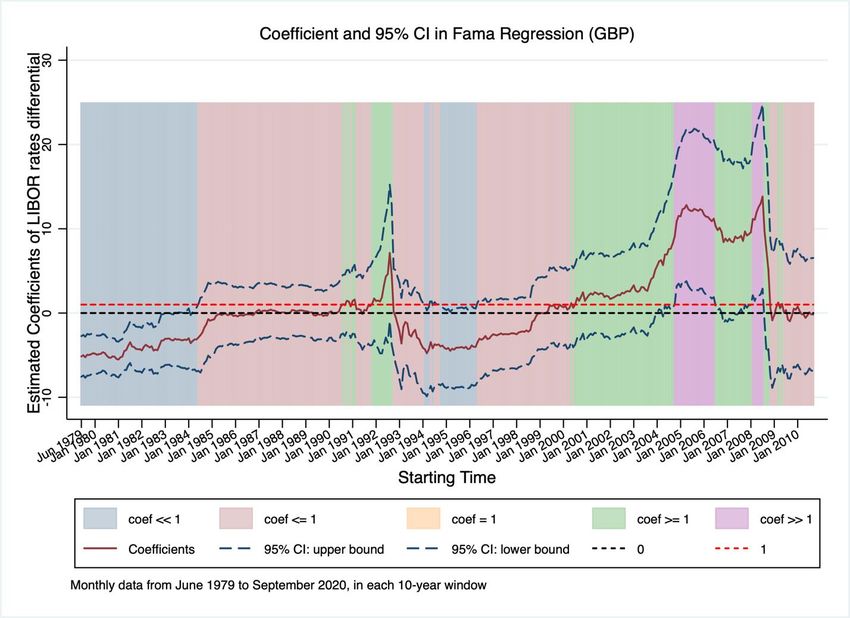
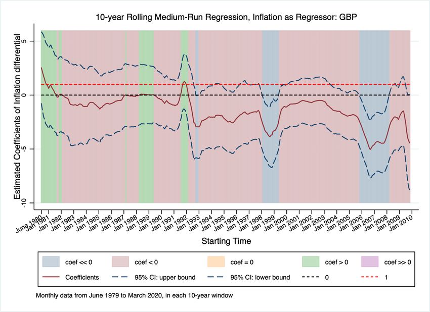
comparable, we have omitted Australia and New Zealand in all the panel estimates. We use the
Driscoll-Kraay (1998) standard error estimates.
 The panel estimate imposes that the slope coefficient is identical across countries (while
allowing the intercept to differ) and will be a more powerful test if the restriction is true. As Table
2 shows, the findings against uncovered interest parity are marginal. The estimated slope
coefficient is -0.14, and the null hypothesis (  = 1 ) can be rejected with a p-value of 0.062. This
finding is consistent with our country-by-country evidence for the 1987:01-2020:09 period. The
null of uncovered interest parity can be weakly rejected.
 In fact, when we split the common sample into the pre-Global Financial Crisis (GFC) and
the period that includes the GFC, we find the slope coefficient estimates are dramatically different.
Table 3 reports estimates of equation (2) for the period 1987:01 – 2006:12, and Table 4 reports the
estimates for the 2007:1 – 2020:09 period. In the earlier period, all the point estimates for the slope
coefficient lie below one, though the 95 percent confidence intervals exclude unity only for CAD,
CHF, JPY, and NZD. In other words, the findings are almost identical to the full sample results
reported in Table 1.11 On the other hand, all the slope coefficients in the later period are estimated
to be positive, but, importantly, the confidence intervals are very wide, and all contain unity.
 The estimates for the panel regressions tell a similar story. On the earlier sample, the slope
coefficient estimate is -0.371, and the null can be weakly rejected, with a p-value of 0.061. But in
the latter period, the point estimate is 4.36, and the standard error of the coefficient estimate is
large (2.84), so the null hypothesis of  = 1 cannot be rejected.
 In Figures 1 – 3, we report estimates of the slope coefficient and 95 percent confidence
intervals using 10-year rolling regressions. For space consideration, we display only the results for
Germany, the U.K. and Japan. These graphs are representative of the findings for all the countries,
and the full set of graphs are presented in the Supplemental Appendix.12 These Figures highlight
the instability of the coefficient estimate of the Fama regression. In the graphs, the dates along the
horizontal axis mark the beginning of each 10-year sample. The blue shaded areas represent the
time periods in which the estimated slope coefficient is significantly less than one at the five
percent level. The pink areas are when the estimated coefficient is less than one, but not

11
 Table 1 reports that the slope coefficient is less than one for the German mark in the full sample, while in the
1989:01 – 2016:12 sample, the 95 percent confidence interval does barely contain one.
12
 We also estimate rolling regressions with 5-year windows. They are similar to those we report in the text with 10-
year windows, but the confidence intervals are wider.

 10

significantly so. The green areas are dates in which the estimated coefficient is greater than one.
The purple areas are times in which the slope coefficient is significantly greater than one at the
five percent level.
 The picture that emerges is fairly incoherent, and that is the important lesson. While the
Fama puzzle is indicated by the findings that the slope coefficient is significantly less than one,
for most of the currencies the time periods over which that is true are relatively short and
concentrated in the pre-2000 period. Most of the time, the 95 percent confidence interval includes
unity. For some of the currencies, such as the New Zealand dollar, there are extended periods of
time for which the estimated coefficient is greater than one.
 In no case is there a sample that starts after January 1999 that has a slope coefficient in the
Fama regression that is less than one. Put another way, no sample that ends after the start of either
the global financial crisis or the start of the very-low interest rate era evinces the Fama puzzle.
 We do not perform joint tests of significance, but it is notable that the estimated slope
coefficients rise during the latter part of the sample for all the currencies. There are two possible
interpretations of these graphs of rolling estimates of the slope coefficient: The first is that the
parameter estimate is very unstable, and there is no true underlying relationship between it − it*

and st +1 − st + it* − it estimated by regression (2). This possibility is consistent with West’s (2012)

observation that the parameter estimate is nearly inconsistent as the discount factor in present value
models of the exchange rate approaches one. The second possibility is that there is a significant
change in the underlying economic relationship between interest rates and excess returns, but we
have not detected statistical significance because we have not used a joint test of significance, and
because the 10-year window is relatively short.
 We performed tests for a structural break in the estimate of the slope coefficient in
regression (2), but, unsurprisingly, the results were quite inconclusive. As evidenced from the
tables and figures, while the value of the slope coefficient has changed greatly over time, the
standard errors of the coefficient estimates in the latter half of the sample are very large. We cannot
reject UIP during this period, but also for most currencies, cannot reject the null of no change in
the slope coefficient.13

13
 We performed Andrews (1993) sup Wald tests for each currency and found significant evidence of a break only
for the Japanese yen, Norwegian krone, New Zealand dollar and Swedish krona.

 11

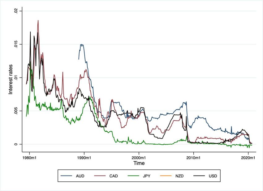
We can ask if there are some regularities in the data that can account for this rise in the
estimated slope coefficient. Figures 4-6 plot the estimated slope coefficients from the 10-year
rolling Fama regressions and the inverse of the variance of it − it* estimated over the same 10-year

time window for Germany, the U.K. and Japan.14
 These graphs show a clear and strong positive correlation between the reciprocal of the
variance of it − it* and the slope coefficient estimates from rolling regressions of equation (2).

Table 5 confirms this by reporting estimates of the correlation between the slope coefficient from
these rolling regressions beginning with 1989:1, and various measures of the volatility of it − it* ,

using both 5-year and 10-year windows.
 What economic forces lead to this pattern of correlations? One explanation that has been
advanced for the puzzling finding of   1 in the Fama regression is that there is a “peso problem”
or the market is incorporating the possibility of a “rare disaster”. Farhi and Gabaix (2016) offer a
model of such a phenomenon. That model posits that high-interest rate currencies incorporate a
risk premium during “good times” because they are currencies that will depreciate greatly during
times of global uncertainty. Thus, the finding of   1 in the Fama regression arises both because
the high-interest-rate currency has a higher expected return than lower-interest-rate currencies, and
because of a peso problem in which the sample that contains only good times does not incorporate
periods in which the high-interest-rate currency has a large depreciation. During bad times, this
same currency has a high interest rate, but the currency depreciates, leading to a slope coefficient
less than one in the Fama regression.
 The Farhi and Gabaix (2016) model could account for our findings. The model produces a
regression coefficient in equation (2), the Fama regression, that is always less than one. If the
sample over which the model is estimated does not include a “disaster”, the slope coefficient
should be negative in their formulation. In the full sample that includes the disaster, the slope
increases, but we should still find   1 , as we do in our full sample. (However, we have noted
that the slope is statistically significantly less than one for fewer than half the countries.)
 Figure 7a-c, however, demonstrates some difficulties with this interpretation for the
variation in the slope coefficient estimate from equation (2) for the U.S. dollar. The figure plots

14
 The graphs for all the countries are in the Supplemental Appendix.

 12

the interest rates for the U.S. and the other countries. The problem, as the graphs illustrate, is that
there is not a sustained period in which the U.S. is either the low-interest-rate currency or the high-
interest-rate currency in the pre-2007 period. In the Farhi and Gabaix (2016) model, the country
with the low interest rate is the less risky country, but if the model is correct, the riskiness of the
country would have to switch frequently as the sign of the interest rate differential switches in the
data. That is, we cannot identify the dollar as, for example, a low-interest-rate currency that is
expected to appreciate during times of global uncertainty. Sometimes its interest rate is lower than
each of the other countries, and sometimes it is higher. The graphs do reveal that the interest rate
of Japan, and to a lesser extent Switzerland, were consistently lower than that of the U.S. pre-
2007, but the puzzling behavior of the slope coefficient in regression (2) applies to U.S. dollar
regressions, not yen or Swiss franc regressions.
 We also can see in Table 6 that the correlation of the slope coefficients from the Fama
regression with the market measure of uncertainty, VIX, are not as high as those reported in Table
5. That is, we would expect under the peso problem/rare disaster explanation a strong negative
correlation between the Fama coefficient and VIX in the 5-year or 10-year moving average, but
that is not the case in fact.
 We tentatively offer a different interpretation. As is well known and confirmed by Figure
7a-c, nominal interest rates in these high-income countries were near zero or below beginning very
soon after the onset of the GFC. At such low levels, interest rates are no longer the most useful
policy instrument for central banks. Instead, central banks implemented a variety of
unconventional policies such as quantitative easing and forward guidance. Our hypothesis is that
the change in the slope coefficient in the Fama regression is related to this change in the principle
monetary policy instrument. Indeed, post-2007, while the slope coefficient estimates are positive,
the confidence intervals are very wide. We think the interest rate differentials may be misleading
guides to the relative monetary policy stance in this era. After 2007, U.S. interest rates, while
historically close to zero, were higher than in most other countries. At the same time, the Federal
Reserve pursued unconventional monetary policies more aggressively than most other countries,
and so their overall stance may have been more accommodative.
 In other words, prior to the GFC, the finding of   1 in equation (2) could be explained
by the models of “delayed reaction” to monetary policy changes. When the Fed, for example,
tightened monetary policy, it , and hence it − it* increased, which led to an immediate appreciation

 13

of the dollar (a drop in st .) However, perhaps because markets did not perceive how persistent the

decline in the interest rate differential would be, or perhaps because expectations are sticky, or
perhaps because portfolio adjustment is costly, or perhaps because of balance sheet constraints,
the initial appreciation was not the maximum appreciation. Exchange rates continued to fall, so
st +1 − st + it* − it fell when it − it* increased. We elaborate on this hypothesis in the concluding

section.
 That same slow reaction to monetary policy changes may have been at work in the post-
2007 era, but monetary policy stance is not well captured by the interest rate differential. To shed
some potential light on the subject, we estimated equation (6). The regressor in this equation is
 t −  t* , the difference in the year-on-year inflation rate in the U.S. relative to the foreign country.
Our notion is this: year-on-year inflation is a proxy for policymakers’ expectations of inflation.
When  t −  t* rises, the U.S. will very soon tighten monetary policy relative to the foreign country.

Then, following the logic of the previous paragraph, delayed reaction by markets leads to high
returns on dollar assets relative to the foreign country, implying a negative slope coefficient in this
regression.
 Table 7 offers some evidence that year-on-year inflation is a reasonable proxy for the stance
of monetary policy. We do not attempt to estimate a Taylor rule for each country, because
measurement of the output gap has been difficult over recent years and is very sensitive to the
methodology. Instead, we estimate (as a panel, with fixed effects, using Driscoll-Kraay standard
errors), the simple and reproducible relationship:
 ic ,t = c ,0 + 1 c ,t +  2ic ,t −1 + uc ,t

where c is the country index. As Table 7 shows, over the entire sample, the estimate of 1 is

positive and significant.15 That is also true for the 1987:01-2006:12 sub-period. But in the ZLB
period, the estimate of 1 is much smaller and is statistically insignificant. This indicates that year-

on-year inflation is a reasonable proxy for monetary policy in the pre-2007 period because interest
rates rise in reaction to higher inflation. In the later period, however, interest rates are no longer

15
 Table 7 also reports results for estimating this equation in the form of G10 country relative to the U.S., but the
conclusions are identical.

 14

the main instrument of monetary policy, but we extrapolate from the earlier period to postulate
that the unconventional policy tools still respond to year-on-year inflation.
 We report estimates for equation (6) for the same time periods as we have for the Fama
regression. As with the Fama regression, these coefficient estimates and standard errors are bias-
corrected using the statistics of Amihud and Hurvich (2004).
 The full-sample results are reported in Table 8. Australia and New Zealand are absent from
this table because those countries do not report monthly inflation rates.
 We can see that all the estimated slope coefficients are negative, with the exception of
France (with a slope of 0.001). Additionally, most are significantly negative at the 5 percent level
(in a two-sided test.) The results are not overwhelmingly strong, allowing for the possibility that
these findings are simply noise, but we note that the fact that all slope coefficients save one are
negative is evidence of a strong pattern.
 Table 9 reports the outcome of estimating equation (6) using the longest common sample,
1987:01 – 2020:09. In this common sample, the findings are quite strong. All the slope coefficient
estimates are negative, and all but two (Japan and Norway) are significantly negative at the five
percent level. The stronger findings over this time period, which excludes the 1980s, relative to
the full sample in reported in Table 8 perhaps reflects the stronger commitment of central banks
to target inflation post-1987:01. The p-value for the panel fixed-effects regression is 0.003,
indicating strong support for the predictive power of relative y.o.y. inflation.
 Importantly, when we look at subsamples of the 1987:01 – 2020:09 period, the story is not
much changed. The number of significant coefficient estimates is reduced because the sample is
shorter, but in both the 1987:01 – 2006:12 period and the 2007:1 – 2020:09 period, the estimated
slope coefficients are all negative (with the sole exception of Japan in the latter period, where the
coefficient is slightly positive), as Tables 10 and 11 demonstrate and most are still statistically
significant at the 5 percent level. The notable point is that there is no qualitative change in these
regressions between the pre-crisis era and the later time period in which unconventional monetary
policies were predominant.
 The panel regression also strongly rejects the null of no predictability for the earlier period,
though does not for the latter period. The panel regression imposes the restriction that the slope
coefficient is the same across all countries, but the estimated coefficient for Japan is positive in

 15

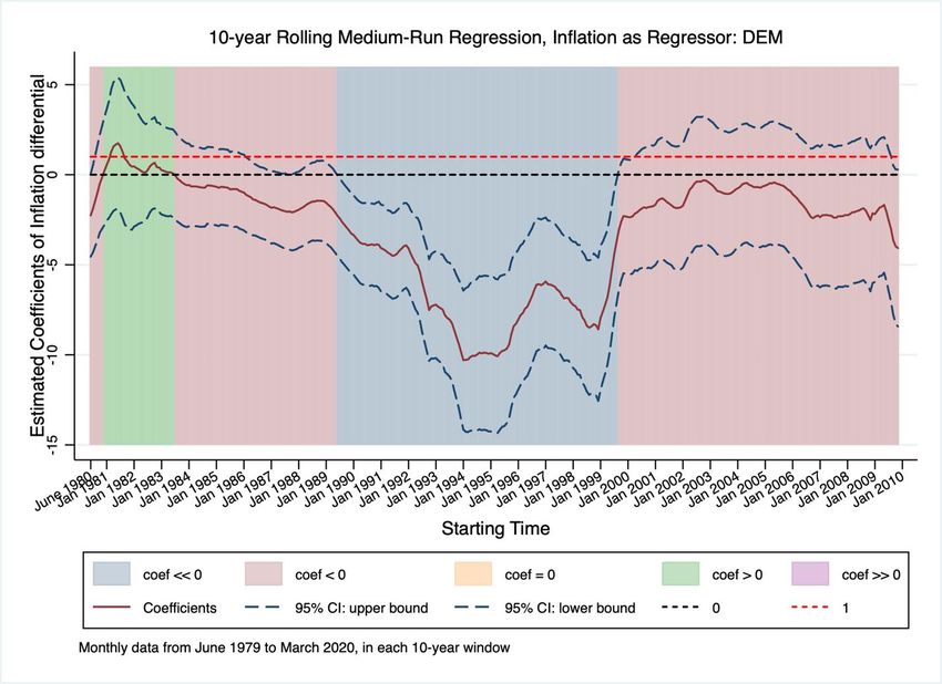
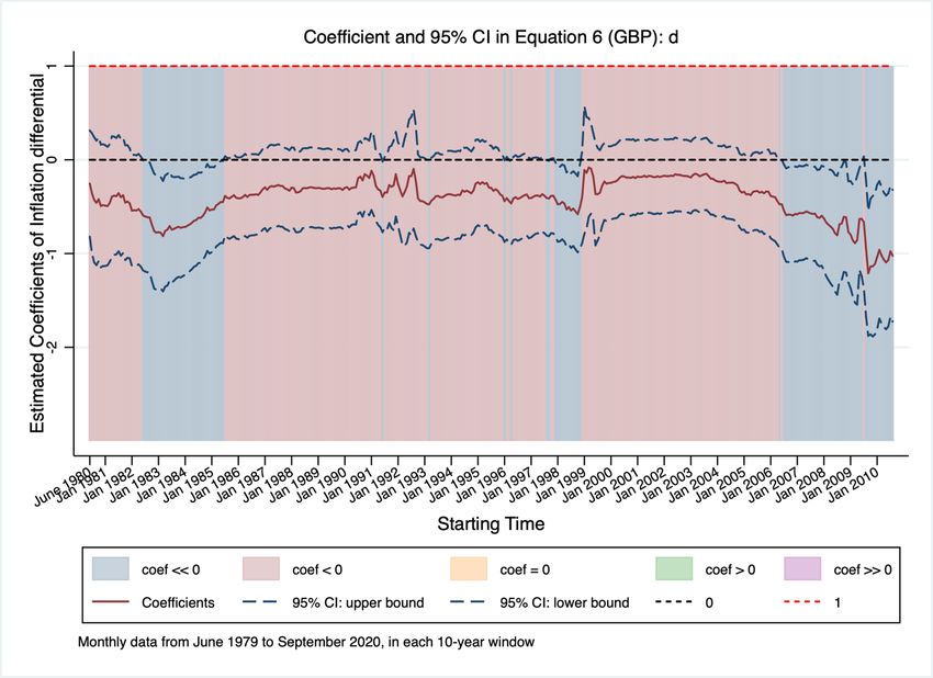
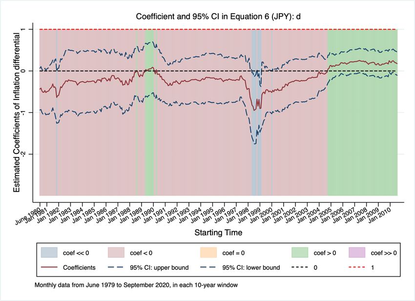
the univariate regressions, in contrast to all the other countries. In turn, this is the main contributor
to the insignificance of the negative coefficient estimated for the panel.
 Figures 8-10 present the slope coefficient estimates from rolling regressions of equation (6)
for Germany, the U.K. and Japan.16 For almost all countries, the coefficient estimates tend to be
consistently negative for all the countries for almost the entire sample after the mid-1980s, with
the major exception being Japan which shows a positive coefficient for the most recent time
periods. In these figures, the dates along the x-axis are the starting dates for each 10-year regression
window. The areas shaded blue are for a slope coefficient that is significantly negative at the 5
percent level. Pink areas represent sample periods for which the slope coefficient is negative but
not significant at the 5 percent level. Green areas are for times of positive coefficient estimates –
none of which are significant at the 5 percent level for any time period.
 The overwhelming impression from these graphs is that the slope coefficient estimates of
equation (6) are negative. There are very few periods of positive coefficients. For a few currencies,
the estimated coefficient is positive for a short window early in the sample (that is, 10-year
estimation windows beginning in the early 1980s.) That window is longer for the Norwegian krone.
The latter part of the sample for the Japanese yen also produces some positive coefficient estimates.
But overall, the picture is clear that higher  t −  t* is associated with lower ex post returns on the

foreign currency, st +1 − st + it* − it . Even during periods in which the Fama puzzle was seen to hold,

prior to 2007, the empirical regularity from this regression is much more consistent. That is, year-
on-year inflation is a better predictor of excess returns than the nominal interest rate differential,
even prior to 2007. However, for many of the countries, the slope coefficient is not significantly
negative at the 5 percent level over many of the subsamples, so it is only tentatively that we
conclude that an increase in inflation abroad tends to predict higher excess returns on foreign
deposits.
 The Supplemental Appendix reports estimates from regressions that include both interest
rate differentials and year-on-year inflation rate differences:

(9) st +1 − st + it* − it =  +  1 ( it − it* ) +  2 ( t −  t* ) + ut +1 .

16
 The figures for all countries are in the Supplemental Appendix.

 16

The econometrics literature does not provide analytical corrections for bias in the coefficient
estimates and standard errors when there is more than one regressor, as is the case here. However,
based on the OLS estimates and Newey-West standard errors, we can draw the following
inferences. First, the evidence for a negative relationship between it − it* and st +1 − st + it* − it is

much weaker when the inflation differential is included in the regression, especially in samples
that begin in the mid-1989s. On the other hand, the evidence for a negative relationship between
 t −  t* and st +1 − st + it* − it remains strong even when it − it* is included in the regression, except
for the three countries of Switzerland, Japan and Norway. This suggests the following
interpretation: The usual finding that the slope coefficient is less than one in the Fama regression,
(2), really is picking up the reaction to monetary policy. The inflation rate over the previous 12
months,  t −  t* is a stronger measure of monetary policy stance than the interest rate differential.

When controlling for year-on-year inflation, there is little evidence of additional explanatory
power from it − it* except perhaps in the 1979-1988 period for currencies for which we have data.

When inflation targeting became more central to monetary policy, both before and after 2007 when
interest rates were very low and unconventional monetary policy became more common, it − it*

has little explanatory power for excess returns once relative inflation is controlled for.
 It is tempting to believe that the significance of the year-on-year inflation differential, along
with the insignificance of the interest rate differential in the zero-lower-bound time period,
suggests that it is the real interest rate differential that predicts excess returns:

(10) ( )
 st +1 − st + it* − it =  + it − it* − Et ( t +1 −  t*+1 ) + ut +1 .

There is immediate reason to be skeptical of this explanation. The puzzle that arises from the
estimation of the Fama equation, (3), is that   0 . If it is, in fact, the real interest rate differential
that matters, we might expect to find   0 in equation (10). But that would mean, holding the
nominal interest rate differential constant (as it nearly is when both countries are near the ZLB),
the effect of the expected inflation differential on the expected return is positive, since from

 ( )
equation (10), Et  t +1 −  t*+1 enters with a negative sign in predicting excess returns. However,

our estimates of the effect of year-on-year inflation on the excess return,  , from equation (6), are

 17

negative. Unless year-on-year inflation predicts the next month’s inflation with a negative sign,
the real interest rate specification in (10) does not account for the significance of year-on-year
inflation in forecasting excess returns, at least not in a way that is consistent with the Fama puzzle.
 To test specification (10), we need a measure of expected inflation in each country. We
implemented this by regressing monthly inflation at time t + 1 on the nominal interest rate and
y.o.y. inflation at time t.17 Using these measures of expected inflation, we construct the real interest
rate differential, and estimate equation (10). Our findings are very similar to the ones with the
nominal interest rate differential as the independent variable, as in the Fama regression. Over the
longest sample, starting in 1980, the estimate of  is negative and significant for most countries.
In the longest common sample, 1987:01-2020:09, we find  is negative and significant for only
Switzerland and Japan. In the pre-ZLB sample, 1987:01-2006:12,  is negative and significant
for those two countries and Canada. In the 2007:01-2020:09 period,  is estimated to be positive
for all countries, though insignificant for all but Italy. Hence, we find the real interest-rate
differential does not consistently predict excess returns, especially during the ZLB period. These
results are reported in detail in the Supplemental Appendix. 18

2. Medium Run

 In this section, we consider estimates of equations (4) and (7). The dependent variable in
these regressions can be interpreted as the return on an investment strategy of buying foreign
exchange, investing in one-month foreign-currency deposits, rolling those deposits over for 12
months then converting the gross investment back into dollars compared to the return from rolling
over one-month dollar deposits for 12 months. Our purpose for looking at the medium horizon is
to assess whether these predicted excess returns are persistent, which may shed further light on
why returns might be predictable.

17
 In fact, we estimated expected inflation of each country relative to the U.S., using as predictors the country/U.S.
relative interest rates and relative year-on-year inflation rates.
18
 The dependent variable in (10) is the “nominal” ex post excess return. The “real” ex post excess return is identical,
except for the addition of the forecast errors of inflation. Those forecast errors should not affect the estimates of the
slope coefficient in (10) because they are uncorrelated with the regressor in (10), as the nominal interest rates are
included in the information set used to make the forecasts of inflation.

 18

These regressions are also subject to the bias in parameter estimates and standard errors
originally noted by Stambaugh (1999) but are also subject to the problems attendant with “long-
horizon” returns regressions. We make use of the bias corrections in the recent study of Boudoukh
et al. (2020), using Newey-West standard errors.
 We consider the same four estimation periods as we did for our short-run return regressions:
the entire sample we have for each country; our longest common sample, 1987:01-2020:09; a pre-
crisis common sample, 1987:01 – 2006:12; and a common sample that includes the low interest
rate era, 2007:01-2020:09.19
 These results are reported in Tables 12–15. For the full sample in Table 12, all the estimated
coefficients are negative, except that for the Italian lira. As the short-term interest differential for
the U.S. relative to the foreign country increases ( it − it* ), the excess return on the foreign

investment falls. These coefficients are significantly less than zero at the five percent level for ten
of the currencies, and at the ten percent level for one more. Only for the Italian lira and Swedish
krona do we fail to reject the null of no predictability at the medium horizon. The findings for this
relationship are much stronger than what we found over the full sample for the short-run returns
in the Fama regression.
 The findings are similar when we use our longest common sample, as reported in Table 13.
Here all the point estimates of the slope coefficient are negative, and seven are significantly less
than zero at the five percent confidence level. The fixed-effects panel regression also finds a
negative slope coefficient that is significant at the 10 percent level. These findings are echoed in
Table 14 for the pre-GFC sample of 1989:01 – 2006:12. All the slope coefficient estimates are
negative, and seven are significantly (at the five percent level) negative. However, the panel
estimate, while negative, is not statistically significant.
 The findings are different in the post-2007:01 sample reported in Table 15. There, five of
the nine estimated coefficients from regression (4) are positive.20 Three are significantly positive
at the five percent level, and none are significantly negative. The slope coefficient in the fixed-
effects panel is positive and significant.
 As with the short-run Fama regressions, before 2007, there is strong evidence of a negative
slope across the currencies, but after 2007 the evidence is mixed. There is no currency that shows

19
 Again, we note that New Zealand’s sample does not begin until 1999.
20
 There are only nine currencies in this period because the euro replaced the mark, French franc and lira.

 19

a significantly negative coefficient in either the short-run or medium-run regressions in the post-
2007 period.
 We also perform rolling regressions, and illustrate the findings in Figures 11-13 for
Germany, the U.K., and Japan, which highlight this sudden shift.21 The horizontal axis gives the
starting date for each 10-year estimation window. The blue-shaded areas represent a slope
coefficient significantly negative at the 5 percent level. Pink areas are for sample periods for which
the slope coefficient is negative but insignificant at the 5 percent level. The area is shaded green
for times of positive coefficient estimates that are not significant, and purple when the coefficient
is positive and significant.
 The graphs all show a large swing in the coefficient estimates in the later part of the sample
compared to the earlier part. For almost all the currencies, that shift begins with 10-year samples
that start in the early 2000s, which coincides with samples in which near-zero interest rates become
predominant. In samples that are primarily drawn from the low-interest rate era, the slope
coefficients are positive, and usually significantly so. We can conclude that we see the same
parameter instability as in the Fama regressions, but with more evidence of a shift in regime from
negative to positive coefficients. That is, the finding of the shift in sign of the slope coefficient is
more likely to be a genuine shift in the relationship rather than just sampling error.
 We turn next to estimates of equation (7), in which excess medium-term returns is again
the dependent variable, and year-on-year inflation is the regressor. We report the slope parameter
estimates and standard errors in Tables 16 – 19 for the different time periods.
 The most striking takeaway from these tables is that all the slope coefficient estimates for
all the currencies and time periods are negative, apart from the French franc and British pound for
the full sample, and Japan in the last sample, which are marginally positive. The French franc and
British pound full sample estimates come from samples that begin in 1979. As we have seen with
the one-month excess returns, the empirical evidence that increases in  t −  t* predict declines in

excess returns on foreign deposits is weaker when the 1980s are included in the sample. If our
working hypothesis is correct, this can be explained by the fact that inflation targeting by central
banks was not as strongly followed in the 1980s as in later periods. That view is perhaps also

21
 The figures for all countries are available in the Supplemental Appendix.

 20

bolstered by the case of Japan in recent years that has found its efforts to boost inflation
unsuccessful and turned to various non-monetary policies such as fiscal expansion.
 In Table 16, which is for the full sample period for each currency, the estimated value of
the slope parameter is strongly significantly negative for six of the nine currencies (and
insignificant but negative for the lira.) In Table 17, which presents evidence for the 1989:01 -
2017:01 period, all parameter estimates are negative, and significantly so at the 5 percent level for
six. For the period 1989:01 – 2006:12, the findings are similar. For the later period when interest
rates were near zero, the coefficient estimates are all negative, though fewer are statistically
significant.
 Figures 14-16 show the slope estimates from rolling regressions with 10-year windows for
Germany, the U.K., and Japan. The figures show that the estimated slope coefficient is negative
almost all of the time for all of the currencies, with very few exceptions. For some currencies,
windows that start in the early 1980s yield positive parameter values, and the Japanese yen shows
a period of positive (but insignificant) parameters at the end of the sample.
 Figures 17-19 (again, for Germany, the U.K., and Japan) offer some perspective into the
channel through which inflation is generating expected excess returns. 22 These charts plot the
parameter estimates of k from the regressions:

(11) ( )
 st +k − st −1 =  + k  t −  t* − ( t −1 −  t*−1 ) +  t +k , k = 0,1,2,

Note that the dependent variable is the change in the exchange rate from time t − 1 to time t + k
(not the change in time t to t + k .) For example, when k = 0 , 0 gives us the association between

the change in the exchange rate between t − 1 and t and changes at time t in the inflation rate
differential.
 We can give a causal explanation to these graphs that is consistent with our hypothesis
about delayed reaction to monetary policy, or underestimation of the persistence of monetary
policy. For each Figure, the first panel shows estimates of (11) for the pre-GFC period of 1989:01
– 2006:12, and the second graph for the period 2007:01 – 2020:09. We find that the k quickly

22
 The graphs for all countries are in the Supplemental Appendix.

 21

turn negative (though not in all cases immediately) as one would expect if monetary policymakers
were targeting inflation, as a tighter monetary policy leads to an appreciation. 23 However, the
maximum appreciation does not occur immediately, but instead many months later. If investors
were adjusting their portfolios continuously to their desired level, and if they had rational
expectations of the persistence of monetary policy, the maximum appreciation should occur as
soon as the market recognizes that policy will be tightened. Although these graphs are not literally
impulse response functions to monetary policy changes or even to news about inflation, they have
that flavor. They show us that exchange rates react slowly to changes in inflation in ways that can
be anticipated. We know that these predictable exchange rate changes are not mirrored in interest
rate changes, and hence there are predictable excess returns.
 We note that the pattern holds well in both periods, pre- and post-2007:01. Even though
the preferred monetary policy instruments changed, the exchange rate reaction to changes in year-
on-year inflation is consistent across time.

3. Long-Run

 To understand the regressions with expected long-run returns as the dependent variable,
equations (5) and (8), take expectations of the “medium-run” regressions. For example, to
motivate (5), begin by taking the expectation at time t of the dependent variable in equation (4),
summing up returns until k periods in the future:

  k 
 Et   st + j +1 − st + j + it*+ j − it + j 
  j =1 

Now subtract the unconditional mean changes in exchange rates, and the unconditional mean
interest rate differential:

 ( ( ))
 k −1
 Et st + k − st − k ( s+1 − s ) − Et  it + j − it*+ j − i − i*
 j =0

Then take the limit as k goes to infinity:

23
 The main exception to this pattern is for Japan, and to a lesser extent for the oil exporters, Canada and Norway.

 22

( ( ))
 
(12) lim  Et st + k − st − k ( s+1 − s )  − Et  it + j − it*+ j − i − i*
 k →   j =0

The term lim  Et st + k − st − k ( s+1 − s )  is (minus) the transitory component of the exchange rate in
 k →  
a Beveridge and Nelson (1981) decomposition. Recall any variable with a unit root can be
decomposed into a component that is a pure random walk, and a component that is transitory. We
shall use a vector autoregression (VAR) to compute a measure of the transitory component of the
exchange rate.
 The second term on the left-hand-side is the “uncovered interest parity level” of the
transitory component of the exchange rate, as defined in Engel (2016). That is, if UIP held, the

 ( ( )) . This can be seen by rearranging the UIP
 
exchange rate would equal to − Et  it + j − it*+ j − i − i*
 j =0

condition, (1), and iterating forward as in Engel (2016). We can also obtain an estimate of this
component from the same VAR mentioned above.
 We then regress the measure obtained for the expression in equation (12) on it − it* as in

equation (5), or on  t −  t* , as in equation (8).

 There are two questions we must address that turn out to be very important for the estimates
of the quantities in (12). First, what variables belong in the VAR that we use to produce the
dependent variable? Second, how important are small sample considerations in the estimate of the
VAR? As it turns out, the two questions are related, and both suggest that results based on shorter
samples may not be very reliable.
 Since we are interested in the response of exchange rates to interest rate changes and
inflation, it seems natural that at a minimum, the VAR that we use should include exchange rates,
interest rates and inflation. A key question, though, is whether we model the real exchange rate as
stationary or not. Define the log of the real exchange rate as qt  st + pt* − pt , where pt is the log

of the consumer price level in the U.S., and pt* is the log of the consumer price level in the foreign

country. There is considerable disagreement in the literature about whether the real exchange rate
is better modeled as converging or as containing a unit root. In fact, Engel (2000) argues that the
question is in essence unresolvable without much longer time series than we use in typical studies.
There are plausible reasons why the real exchange rate may be stationary but converging very
slowly so that it appears to have a unit root when it does not. Conversely, even if one rejects a unit
 23