A Style-Based Generator Architecture for Generative Adversarial Networks
←
→
Page content transcription
If your browser does not render page correctly, please read the page content below
A Style-Based Generator Architecture for Generative Adversarial Networks

                                                                  Tero Karras                       Samuli Laine                        Timo Aila
                                                                   NVIDIA                             NVIDIA                            NVIDIA
                                                             tkarras@nvidia.com                  slaine@nvidia.com                 taila@nvidia.com
arXiv:1812.04948v3 [cs.NE] 29 Mar 2019

                                                                  Abstract                                      (e.g., pose, identity) from stochastic variation (e.g., freck-
                                                                                                                les, hair) in the generated images, and enables intuitive
                                             We propose an alternative generator architecture for               scale-specific mixing and interpolation operations. We do
                                         generative adversarial networks, borrowing from style                  not modify the discriminator or the loss function in any
                                         transfer literature. The new architecture leads to an au-              way, and our work is thus orthogonal to the ongoing discus-
                                         tomatically learned, unsupervised separation of high-level             sion about GAN loss functions, regularization, and hyper-
                                         attributes (e.g., pose and identity when trained on human              parameters [24, 45, 5, 40, 44, 36].
                                         faces) and stochastic variation in the generated images                    Our generator embeds the input latent code into an inter-
                                         (e.g., freckles, hair), and it enables intuitive, scale-specific       mediate latent space, which has a profound effect on how
                                         control of the synthesis. The new generator improves the               the factors of variation are represented in the network. The
                                         state-of-the-art in terms of traditional distribution quality          input latent space must follow the probability density of the
                                         metrics, leads to demonstrably better interpolation proper-            training data, and we argue that this leads to some degree of
                                         ties, and also better disentangles the latent factors of varia-        unavoidable entanglement. Our intermediate latent space
                                         tion. To quantify interpolation quality and disentanglement,           is free from that restriction and is therefore allowed to be
                                         we propose two new, automated methods that are applica-                disentangled. As previous methods for estimating the de-
                                         ble to any generator architecture. Finally, we introduce a             gree of latent space disentanglement are not directly appli-
                                         new, highly varied and high-quality dataset of human faces.            cable in our case, we propose two new automated metrics —
                                                                                                                perceptual path length and linear separability — for quanti-
                                                                                                                fying these aspects of the generator. Using these metrics, we
                                                                                                                show that compared to a traditional generator architecture,
                                         1. Introduction                                                        our generator admits a more linear, less entangled represen-
                                                                                                                tation of different factors of variation.
                                            The resolution and quality of images produced by gen-                   Finally, we present a new dataset of human faces
                                         erative methods — especially generative adversarial net-               (Flickr-Faces-HQ, FFHQ) that offers much higher qual-
                                         works (GAN) [22] — have seen rapid improvement recently                ity and covers considerably wider variation than existing
                                         [30, 45, 5]. Yet the generators continue to operate as black           high-resolution datasets (Appendix A). We have made this
                                         boxes, and despite recent efforts [3], the understanding of            dataset publicly available, along with our source code and
                                         various aspects of the image synthesis process, e.g., the ori-         pre-trained networks.1 The accompanying video can be
                                         gin of stochastic features, is still lacking. The properties of        found under the same link.
                                         the latent space are also poorly understood, and the com-
                                         monly demonstrated latent space interpolations [13, 52, 37]
                                         provide no quantitative way to compare different generators            2. Style-based generator
                                         against each other.                                                        Traditionally the latent code is provided to the genera-
                                            Motivated by style transfer literature [27], we re-design           tor through an input layer, i.e., the first layer of a feed-
                                         the generator architecture in a way that exposes novel ways            forward network (Figure 1a). We depart from this design
                                         to control the image synthesis process. Our generator starts           by omitting the input layer altogether and starting from a
                                         from a learned constant input and adjusts the “style” of               learned constant instead (Figure 1b, right). Given a latent
                                         the image at each convolution layer based on the latent                code z in the input latent space Z, a non-linear mapping
                                         code, therefore directly controlling the strength of image             network f : Z → W first produces w ∈ W (Figure 1b,
                                         features at different scales. Combined with noise injected             left). For simplicity, we set the dimensionality of both
                                         directly into the network, this architectural change leads to
                                         automatic, unsupervised separation of high-level attributes              1 https://github.com/NVlabs/stylegan

                                                                                                            1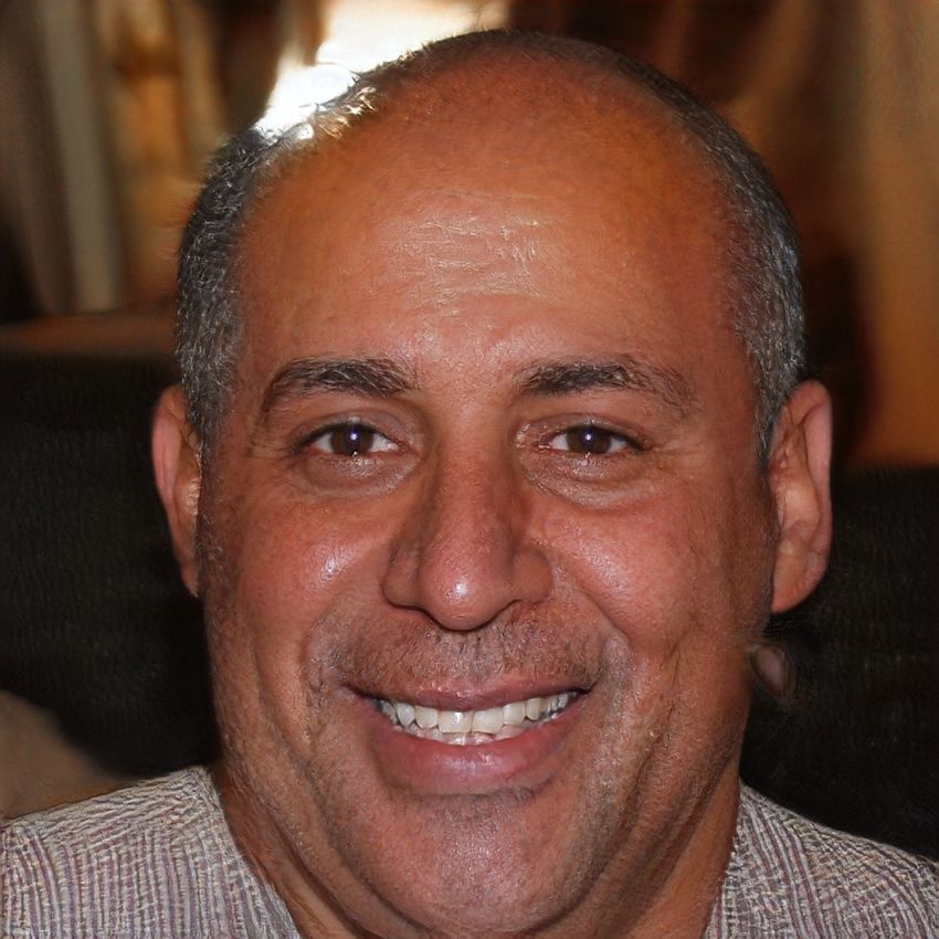
Latent               Latent                                             Noise            Method                              CelebA-HQ       FFHQ
                                             Synthesis network
                                                                                      A   Baseline Progressive GAN [30]         7.79           8.04
    Normalize           Normalize               Const 4×4×512                         B   + Tuning (incl. bilinear up/down)     6.11           5.25
                               Mapping                               B
                                               style                                  C   + Add mapping and styles              5.34           4.85
 Fully-connected               network     A           AdaIN                          D   + Remove traditional input            5.07           4.88
   PixelNorm               FC                      Conv 3×3                           E   + Add noise inputs                    5.06           4.42
    Conv 3×3               FC                                        B                F   + Mixing regularization               5.17           4.40
                                               style
   PixelNorm               FC              A           AdaIN
                                                               4×4
                4×4        FC                                                        Table 1. Fréchet inception distance (FID) for various generator de-
                           FC                                                        signs (lower is better). In this paper we calculate the FIDs using
                                                   Upsample
    Upsample               FC                                                        50,000 images drawn randomly from the training set, and report
                                                   Conv 3×3
    Conv 3×3               FC                                                        the lowest distance encountered over the course of training.
                                                                     B
                           FC                  style
   PixelNorm                               A           AdaIN
    Conv 3×3                                       Conv 3×3                             Finally, we provide our generator with a direct means
   PixelNorm                                   style
                                                                     B               to generate stochastic detail by introducing explicit noise
                                           A           AdaIN                         inputs. These are single-channel images consisting of un-
                8×8                                            8×8
                                                                                     correlated Gaussian noise, and we feed a dedicated noise
                                                                                     image to each layer of the synthesis network. The noise
 (a) Traditional                 (b) Style-based generator                           image is broadcasted to all feature maps using learned per-
Figure 1. While a traditional generator [30] feeds the latent code                   feature scaling factors and then added to the output of the
though the input layer only, we first map the input to an in-                        corresponding convolution, as illustrated in Figure 1b. The
termediate latent space W, which then controls the generator                         implications of adding the noise inputs are discussed in Sec-
through adaptive instance normalization (AdaIN) at each convo-                       tions 3.2 and 3.3.
lution layer. Gaussian noise is added after each convolution, be-
fore evaluating the nonlinearity. Here “A” stands for a learned                      2.1. Quality of generated images
affine transform, and “B” applies learned per-channel scaling fac-
                                                                                         Before studying the properties of our generator, we
tors to the noise input. The mapping network f consists of 8 lay-
ers and the synthesis network g consists of 18 layers — two for                      demonstrate experimentally that the redesign does not com-
each resolution (42 − 10242 ). The output of the last layer is con-                  promise image quality but, in fact, improves it considerably.
verted to RGB using a separate 1 × 1 convolution, similar to Kar-                    Table 1 gives Fréchet inception distances (FID) [25] for var-
ras et al. [30]. Our generator has a total of 26.2M trainable param-                 ious generator architectures in C ELEBA-HQ [30] and our
eters, compared to 23.1M in the traditional generator.                               new FFHQ dataset (Appendix A). Results for other datasets
                                                                                     are given in Appendix E. Our baseline configuration (A)
spaces to 512, and the mapping f is implemented using                                is the Progressive GAN setup of Karras et al. [30], from
an 8-layer MLP, a decision we will analyze in Section 4.1.                           which we inherit the networks and all hyperparameters ex-
Learned affine transformations then specialize w to styles                           cept where stated otherwise. We first switch to an improved
y = (ys , yb ) that control adaptive instance normalization                          baseline (B) by using bilinear up/downsampling operations
(AdaIN) [27, 17, 21, 16] operations after each convolution                           [64], longer training, and tuned hyperparameters. A de-
layer of the synthesis network g. The AdaIN operation is                             tailed description of training setups and hyperparameters is
defined as                                                                           included in Appendix C. We then improve this new base-
                                                                                     line further by adding the mapping network and AdaIN op-
                                     xi − µ(xi )
           AdaIN(xi , y) = ys,i                  + yb,i ,                 (1)        erations (C), and make a surprising observation that the net-
                                        σ(xi )                                       work no longer benefits from feeding the latent code into the
where each feature map xi is normalized separately, and                              first convolution layer. We therefore simplify the architec-
then scaled and biased using the corresponding scalar com-                           ture by removing the traditional input layer and starting the
ponents from style y. Thus the dimensionality of y is twice                          image synthesis from a learned 4 × 4 × 512 constant tensor
the number of feature maps on that layer.                                            (D). We find it quite remarkable that the synthesis network
   Comparing our approach to style transfer, we compute                              is able to produce meaningful results even though it receives
the spatially invariant style y from vector w instead of an                          input only through the styles that control the AdaIN opera-
example image. We choose to reuse the word “style” for                               tions.
y because similar network architectures are already used                                 Finally, we introduce the noise inputs (E) that improve
for feedforward style transfer [27], unsupervised image-to-                          the results further, as well as novel mixing regularization (F)
image translation [28], and domain mixtures [23]. Com-                               that decorrelates neighboring styles and enables more fine-
pared to more general feature transforms [38, 57], AdaIN is                          grained control over the generated imagery (Section 3.1).
particularly well suited for our purposes due to its efficiency                          We evaluate our methods using two different loss func-
and compact representation.                                                          tions: for C ELEBA-HQ we rely on WGAN-GP [24],

                                                                                 2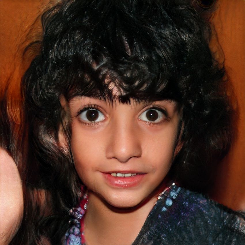
2.2. Prior art
                                                                                Much of the work on GAN architectures has focused
                                                                            on improving the discriminator by, e.g., using multiple
                                                                            discriminators [18, 47, 11], multiresolution discrimination
                                                                            [60, 55], or self-attention [63]. The work on generator side
                                                                            has mostly focused on the exact distribution in the input la-
                                                                            tent space [5] or shaping the input latent space via Gaussian
                                                                            mixture models [4], clustering [48], or encouraging convex-
                                                                            ity [52].
                                                                                Recent conditional generators feed the class identifier
                                                                            through a separate embedding network to a large number
                                                                            of layers in the generator [46], while the latent is still pro-
                                                                            vided though the input layer. A few authors have considered
                                                                            feeding parts of the latent code to multiple generator layers
                                                                            [9, 5]. In parallel work, Chen et al. [6] “self modulate” the
                                                                            generator using AdaINs, similarly to our work, but do not
                                                                            consider an intermediate latent space or noise inputs.

                                                                            3. Properties of the style-based generator
                                                                                Our generator architecture makes it possible to control
                                                                            the image synthesis via scale-specific modifications to the
                                                                            styles. We can view the mapping network and affine trans-
                                                                            formations as a way to draw samples for each style from a
                                                                            learned distribution, and the synthesis network as a way to
                                                                            generate a novel image based on a collection of styles. The
Figure 2. Uncurated set of images produced by our style-based               effects of each style are localized in the network, i.e., modi-
generator (config F) with the FFHQ dataset. Here we used a varia-           fying a specific subset of the styles can be expected to affect
tion of the truncation trick [42, 5, 34] with ψ = 0.7 for resolutions       only certain aspects of the image.
42 − 322 . Please see the accompanying video for more results.                  To see the reason for this localization, let us consider
                                                                            how the AdaIN operation (Eq. 1) first normalizes each chan-
while FFHQ uses WGAN-GP for configuration A and non-                        nel to zero mean and unit variance, and only then applies
saturating loss [22] with R1 regularization [44, 51, 14] for                scales and biases based on the style. The new per-channel
configurations B–F. We found these choices to give the best                 statistics, as dictated by the style, modify the relative impor-
results. Our contributions do not modify the loss function.                 tance of features for the subsequent convolution operation,
   We observe that the style-based generator (E) improves                   but they do not depend on the original statistics because of
FIDs quite significantly over the traditional generator (B),                the normalization. Thus each style controls only one convo-
almost 20%, corroborating the large-scale ImageNet mea-                     lution before being overridden by the next AdaIN operation.
surements made in parallel work [6, 5]. Figure 2 shows an
                                                                            3.1. Style mixing
uncurated set of novel images generated from the FFHQ
dataset using our generator. As confirmed by the FIDs,                         To further encourage the styles to localize, we employ
the average quality is high, and even accessories such                      mixing regularization, where a given percentage of images
as eyeglasses and hats get successfully synthesized. For                    are generated using two random latent codes instead of one
this figure, we avoided sampling from the extreme regions                   during training. When generating such an image, we sim-
of W using the so-called truncation trick [42, 5, 34] —                     ply switch from one latent code to another — an operation
Appendix B details how the trick can be performed in W                      we refer to as style mixing — at a randomly selected point
instead of Z. Note that our generator allows applying the                   in the synthesis network. To be specific, we run two latent
truncation selectively to low resolutions only, so that high-               codes z1 , z2 through the mapping network, and have the
resolution details are not affected.                                        corresponding w1 , w2 control the styles so that w1 applies
   All FIDs in this paper are computed without the trun-                    before the crossover point and w2 after it. This regular-
cation trick, and we only use it for illustrative purposes in               ization technique prevents the network from assuming that
Figure 2 and the video. All images are generated in 10242                   adjacent styles are correlated.
resolution.                                                                    Table 2 shows how enabling mixing regularization dur-

                                                                        3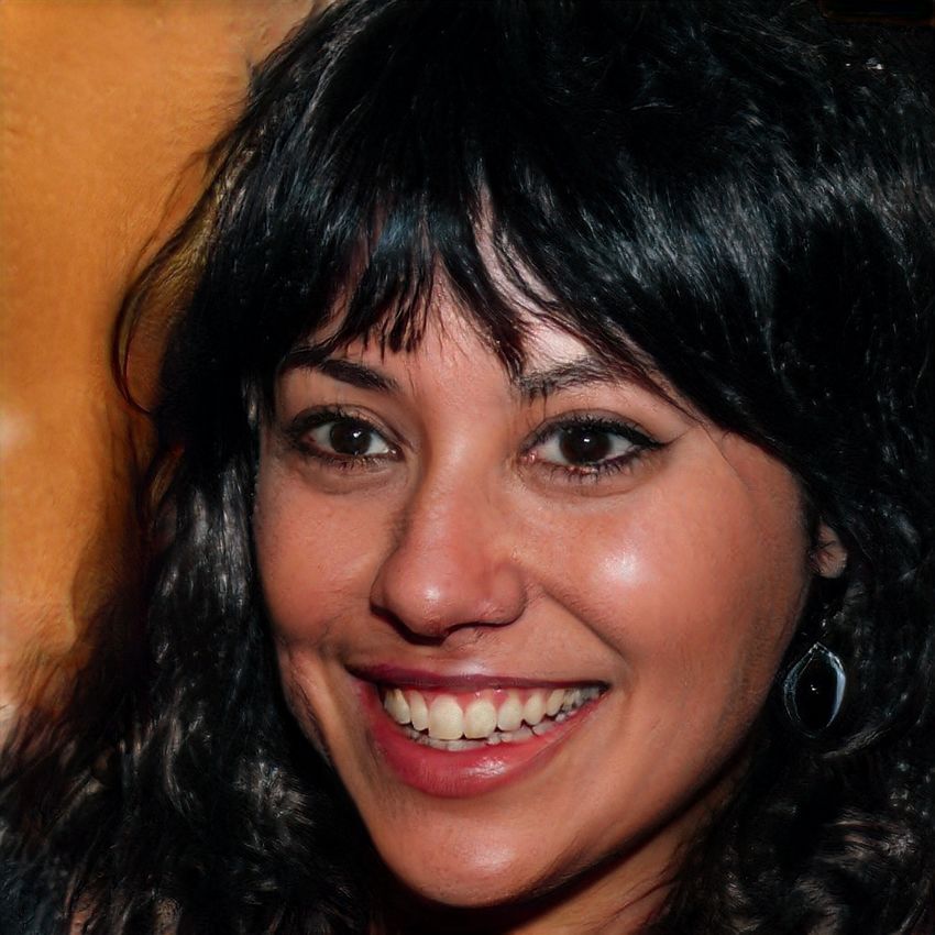
Source A   Source B
 Coarse styles from source B
 Middle styles from source B
    Fine from B

Figure 3. Two sets of images were generated from their respective latent codes (sources A and B); the rest of the images were generated by
copying a specified subset of styles from source B and taking the rest from source A. Copying the styles corresponding to coarse spatial
resolutions (42 – 82 ) brings high-level aspects such as pose, general hair style, face shape, and eyeglasses from source B, while all colors
(eyes, hair, lighting) and finer facial features resemble A. If we instead copy the styles of middle resolutions (162 – 322 ) from B, we inherit
smaller scale facial features, hair style, eyes open/closed from B, while the pose, general face shape, and eyeglasses from A are preserved.
Finally, copying the fine styles (642 – 10242 ) from B brings mainly the color scheme and microstructure.

                                                                       4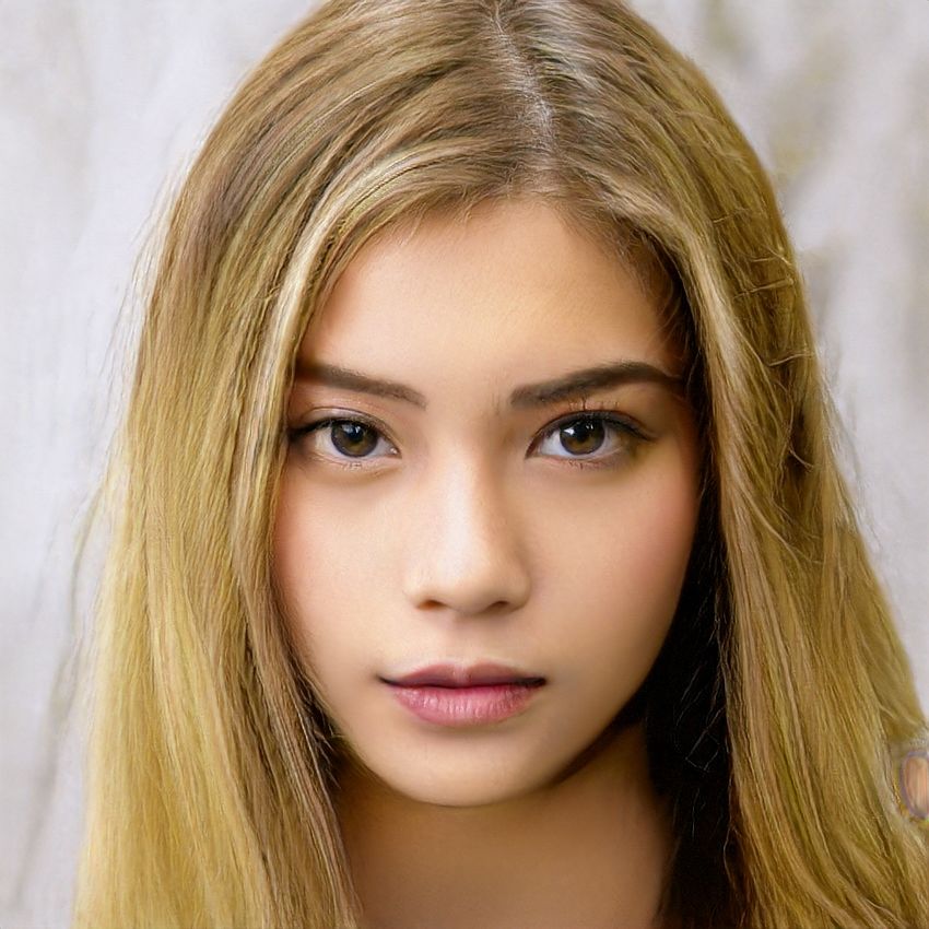
Mixing                  Number of latents during testing
      regularization      1           2            3           4
  E 0%                  4.42         8.22        12.88        17.41
    50%                 4.41         6.10         8.71        11.61
  F 90%                 4.40         5.11         6.88         9.03
    100%                4.83         5.17         6.63         8.40

Table 2. FIDs in FFHQ for networks trained by enabling the mix-
ing regularization for different percentage of training examples.
Here we stress test the trained networks by randomizing 1 . . . 4
latents and the crossover points between them. Mixing regular-                      (a)               (b)
ization improves the tolerance to these adverse operations signifi-
cantly. Labels E and F refer to the configurations in Table 1.

                                                                                    (c)               (d)

                                                                              Figure 5. Effect of noise inputs at different layers of our genera-
                                                                              tor. (a) Noise is applied to all layers. (b) No noise. (c) Noise in
                                                                              fine layers only (642 – 10242 ). (d) Noise in coarse layers only
                                                                              (42 – 322 ). We can see that the artificial omission of noise leads to
                                                                              featureless “painterly” look. Coarse noise causes large-scale curl-
 (a) Generated image    (b) Stochastic variation (c) Standard deviation       ing of hair and appearance of larger background features, while
                                                                              the fine noise brings out the finer curls of hair, finer background
Figure 4. Examples of stochastic variation. (a) Two generated                 detail, and skin pores.
images. (b) Zoom-in with different realizations of input noise.
While the overall appearance is almost identical, individual hairs
are placed very differently. (c) Standard deviation of each pixel             from earlier activations whenever they are needed. This
over 100 different realizations, highlighting which parts of the im-          consumes network capacity and hiding the periodicity of
ages are affected by the noise. The main areas are the hair, silhou-          generated signal is difficult — and not always successful, as
ettes, and parts of background, but there is also interesting stochas-        evidenced by commonly seen repetitive patterns in gener-
tic variation in the eye reflections. Global aspects such as identity
                                                                              ated images. Our architecture sidesteps these issues alto-
and pose are unaffected by stochastic variation.
                                                                              gether by adding per-pixel noise after each convolution.
                                                                                  Figure 4 shows stochastic realizations of the same un-
ing training improves the localization considerably, indi-                    derlying image, produced using our generator with differ-
cated by improved FIDs in scenarios where multiple latents                    ent noise realizations. We can see that the noise affects only
are mixed at test time. Figure 3 presents examples of images                  the stochastic aspects, leaving the overall composition and
synthesized by mixing two latent codes at various scales.                     high-level aspects such as identity intact. Figure 5 further
We can see that each subset of styles controls meaningful                     illustrates the effect of applying stochastic variation to dif-
high-level attributes of the image.                                           ferent subsets of layers. Since these effects are best seen
                                                                              in animation, please consult the accompanying video for a
3.2. Stochastic variation
                                                                              demonstration of how changing the noise input of one layer
   There are many aspects in human portraits that can be                      leads to stochastic variation at a matching scale.
regarded as stochastic, such as the exact placement of hairs,                     We find it interesting that the effect of noise appears
stubble, freckles, or skin pores. Any of these can be ran-                    tightly localized in the network. We hypothesize that at any
domized without affecting our perception of the image as                      point in the generator, there is pressure to introduce new
long as they follow the correct distribution.                                 content as soon as possible, and the easiest way for our net-
   Let us consider how a traditional generator implements                     work to create stochastic variation is to rely on the noise
stochastic variation. Given that the only input to the net-                   provided. A fresh set of noise is available for every layer,
work is through the input layer, the network needs to invent                  and thus there is no incentive to generate the stochastic ef-
a way to generate spatially-varying pseudorandom numbers                      fects from earlier activations, leading to a localized effect.

                                                                          5
pling according to any fixed distribution; its sampling den-
                                                                                   sity is induced by the learned piecewise continuous map-
                                                                                   ping f (z). This mapping can be adapted to “unwarp” W so
                                                                                   that the factors of variation become more linear. We posit
                                                                                   that there is pressure for the generator to do so, as it should
                                                                                   be easier to generate realistic images based on a disentan-
   (a) Distribution of      (b) Mapping from          (c) Mapping from             gled representation than based on an entangled representa-
 features in training set     Z to features             W to features
                                                                                   tion. As such, we expect the training to yield a less entan-
Figure 6. Illustrative example with two factors of variation (im-                  gled W in an unsupervised setting, i.e., when the factors of
age features, e.g., masculinity and hair length). (a) An example                   variation are not known in advance [10, 35, 49, 8, 26, 32, 7].
training set where some combination (e.g., long haired males) is                       Unfortunately the metrics recently proposed for quanti-
missing. (b) This forces the mapping from Z to image features to
                                                                                   fying disentanglement [26, 32, 7, 19] require an encoder
become curved so that the forbidden combination disappears in Z
                                                                                   network that maps input images to latent codes. These met-
to prevent the sampling of invalid combinations. (c) The learned
mapping from Z to W is able to “undo” much of the warping.                         rics are ill-suited for our purposes since our baseline GAN
                                                                                   lacks such an encoder. While it is possible to add an extra
                                                                                   network for this purpose [8, 12, 15], we want to avoid in-
3.3. Separation of global effects from stochasticity                               vesting effort into a component that is not a part of the actual
                                                                                   solution. To this end, we describe two new ways of quanti-
    The previous sections as well as the accompanying video                        fying disentanglement, neither of which requires an encoder
demonstrate that while changes to the style have global ef-                        or known factors of variation, and are therefore computable
fects (changing pose, identity, etc.), the noise affects only                      for any image dataset and generator.
inconsequential stochastic variation (differently combed
hair, beard, etc.). This observation is in line with style trans-                  4.1. Perceptual path length
fer literature, where it has been established that spatially
                                                                                       As noted by Laine [37], interpolation of latent-space vec-
invariant statistics (Gram matrix, channel-wise mean, vari-
                                                                                   tors may yield surprisingly non-linear changes in the image.
ance, etc.) reliably encode the style of an image [20, 39]
                                                                                   For example, features that are absent in either endpoint may
while spatially varying features encode a specific instance.
                                                                                   appear in the middle of a linear interpolation path. This is
    In our style-based generator, the style affects the entire
                                                                                   a sign that the latent space is entangled and the factors of
image because complete feature maps are scaled and bi-
                                                                                   variation are not properly separated. To quantify this ef-
ased with the same values. Therefore, global effects such
                                                                                   fect, we can measure how drastic changes the image under-
as pose, lighting, or background style can be controlled co-
                                                                                   goes as we perform interpolation in the latent space. Intu-
herently. Meanwhile, the noise is added independently to
                                                                                   itively, a less curved latent space should result in perceptu-
each pixel and is thus ideally suited for controlling stochas-
                                                                                   ally smoother transition than a highly curved latent space.
tic variation. If the network tried to control, e.g., pose using
                                                                                       As a basis for our metric, we use a perceptually-based
the noise, that would lead to spatially inconsistent decisions
                                                                                   pairwise image distance [65] that is calculated as a weighted
that would then be penalized by the discriminator. Thus the
                                                                                   difference between two VGG16 [58] embeddings, where
network learns to use the global and local channels appro-
                                                                                   the weights are fit so that the metric agrees with human per-
priately, without explicit guidance.
                                                                                   ceptual similarity judgments. If we subdivide a latent space
                                                                                   interpolation path into linear segments, we can define the
4. Disentanglement studies                                                         total perceptual length of this segmented path as the sum
    There are various definitions for disentanglement [54,                         of perceptual differences over each segment, as reported by
50, 2, 7, 19], but a common goal is a latent space that con-                       the image distance metric. A natural definition for the per-
sists of linear subspaces, each of which controls one fac-                         ceptual path length would be the limit of this sum under
tor of variation. However, the sampling probability of each                        infinitely fine subdivision, but in practice we approximate it
combination of factors in Z needs to match the correspond-                         using a small subdivision epsilon  = 10−4 . The average
ing density in the training data. As illustrated in Figure 6,                      perceptual path length in latent space Z, over all possible
this precludes the factors from being fully disentangled with                      endpoints, is therefore
typical datasets and input latent distributions.2                                                    h1
    A major benefit of our generator architecture is that the                                lZ = E 2 d G(slerp(z1 , z2 ; t)),
                                                                                                                                    i       (2)
intermediate latent space W does not have to support sam-                                                   G(slerp(z1 , z2 ; t + )) ,
   2 The few artificial datasets designed for disentanglement studies (e.g.,

[43, 19]) tabulate all combinations of predetermined factors of variation          where z1 , z2 ∼ P (z), t ∼ U (0, 1), G is the generator (i.e.,
with uniform frequency, thus hiding the problem.                                   g ◦ f for style-based networks), and d(·, ·) evaluates the per-

                                                                               6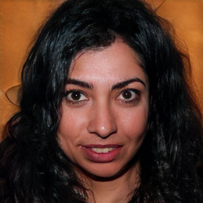
Path length         Separa-                                                  Path length       Separa-
      Method                                                                     Method             FID
                                  full         end        bility                                                full       end       bility
  B Traditional generator   Z    412.0        415.3       10.78              B Traditional 0   Z    5.25       412.0      415.3       10.78
  D Style-based generator   W    446.2        376.6        3.61                Traditional 8   Z    4.87       896.2      902.0      170.29
  E + Add noise inputs      W    200.5        160.6        3.54                Traditional 8   W    4.87       324.5      212.2        6.52
    + Mixing 50%            W    231.5        182.1        3.51                Style-based 0   Z    5.06       283.5      285.5        9.88
  F + Mixing 90%            W    234.0        195.9        3.79                Style-based 1   W    4.60       219.9      209.4        6.81
                                                                               Style-based 2   W    4.43       217.8      199.9        6.25
Table 3. Perceptual path lengths and separability scores for various         F Style-based 8   W    4.40       234.0      195.9        3.79
generator architectures in FFHQ (lower is better). We perform the
measurements in Z for the traditional network, and in W for style-         Table 4. The effect of a mapping network in FFHQ. The number
based ones. Making the network resistant to style mixing appears           in method name indicates the depth of the mapping network. We
to distort the intermediate latent space W somewhat. We hypothe-           see that FID, separability, and path length all benefit from having
size that mixing makes it more difficult for W to efficiently encode       a mapping network, and this holds for both style-based and tra-
factors of variation that span multiple scales.                            ditional generator architectures. Furthermore, a deeper mapping
                                                                           network generally performs better than a shallow one.

ceptual distance between the resulting images. Here slerp
denotes spherical interpolation [56], which is the most ap-                4.2. Linear separability
propriate way of interpolating in our normalized input latent                  If a latent space is sufficiently disentangled, it should
space [61]. To concentrate on the facial features instead of               be possible to find direction vectors that consistently corre-
background, we crop the generated images to contain only                   spond to individual factors of variation. We propose another
the face prior to evaluating the pairwise image metric. As                 metric that quantifies this effect by measuring how well the
the metric d is quadratic [65], we divide by 2 . We compute               latent-space points can be separated into two distinct sets
the expectation by taking 100,000 samples.                                 via a linear hyperplane, so that each set corresponds to a
   Computing the average perceptual path length in W is                    specific binary attribute of the image.
carried out in a similar fashion:                                              In order to label the generated images, we train auxiliary
               h1                                                          classification networks for a number of binary attributes,
      lW = E 2 d g(lerp(f (z1 ), f (z2 ); t)),                             e.g., to distinguish male and female faces. In our tests,
                                                    i   (3)
                     g(lerp(f (z1 ), f (z2 ); t + )) ,                    the classifiers had the same architecture as the discrimina-
                                                                           tor we use (i.e., same as in [30]), and were trained using the
where the only difference is that interpolation happens in                 C ELEBA-HQ dataset that retains the 40 attributes available
W space. Because vectors in W are not normalized in any                    in the original CelebA dataset. To measure the separability
fashion, we use linear interpolation (lerp).                               of one attribute, we generate 200,000 images with z ∼ P (z)
    Table 3 shows that this full-path length is substantially              and classify them using the auxiliary classification network.
shorter for our style-based generator with noise inputs, in-               We then sort the samples according to classifier confidence
dicating that W is perceptually more linear than Z. Yet, this              and remove the least confident half, yielding 100,000 la-
measurement is in fact slightly biased in favor of the input               beled latent-space vectors.
latent space Z. If W is indeed a disentangled and “flat-                       For each attribute, we fit a linear SVM to predict the label
tened” mapping of Z, it may contain regions that are not on                based on the latent-space point — z for traditional and w for
the input manifold — and are thus badly reconstructed by                   style-based — and classify the points by this plane. We then
the generator — even between points that are mapped from                   compute the conditional entropy H(Y |X) where X are the
the input manifold, whereas the input latent space Z has no                classes predicted by the SVM and Y are the classes deter-
such regions by definition. It is therefore to be expected that            mined by the pre-trained classifier. This tells how much ad-
if we restrict our measure to path endpoints, i.e., t ∈ {0, 1},            ditional information is required to determine the true class
we should obtain a smaller lW while lZ is not affected. This               of a sample, given that we know on which side of the hy-
is indeed what we observe in Table 3.                                      perplane it lies. A low value suggests consistent latent space
    Table 4 shows how path lengths are affected by the map-                directions for the corresponding factor(s) of variation.
ping network. We see that both traditional and style-based                     WeP calculate the final separability score as
generators benefit from having a mapping network, and ad-                  exp( i H(Yi |Xi )), where i enumerates the 40 attributes.
ditional depth generally improves the perceptual path length               Similar to the inception score [53], the exponentiation
as well as FIDs. It is interesting that while lW improves in               brings the values from logarithmic to linear domain so that
the traditional generator, lZ becomes considerably worse,                  they are easier to compare.
illustrating our claim that the input latent space can indeed                  Tables 3 and 4 show that W is consistently better sep-
be arbitrarily entangled in GANs.                                          arable than Z, suggesting a less entangled representation.

                                                                       7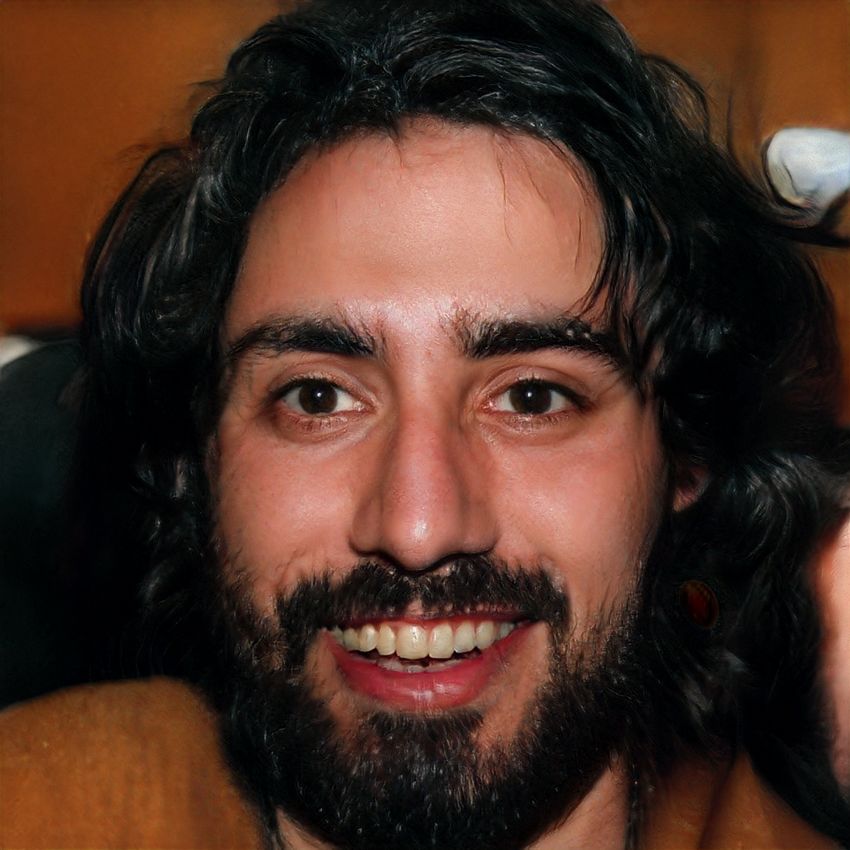
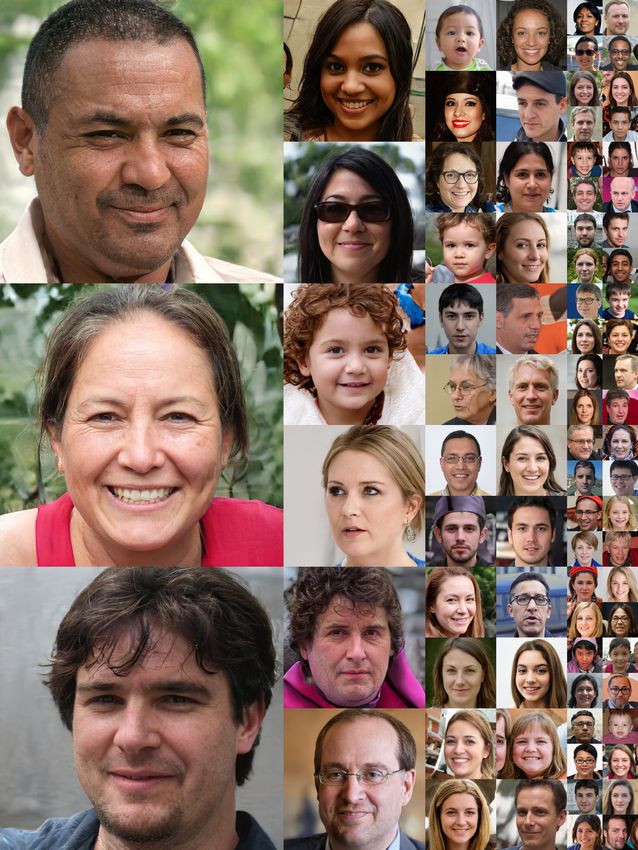
Figure 7. The FFHQ dataset offers a lot of variety in terms of age, ethnicity, viewpoint, lighting, and image background.

Furthermore, increasing the depth of the mapping network
improves both image quality and separability in W, which
is in line with the hypothesis that the synthesis network in-
herently favors a disentangled input representation. Inter-
estingly, adding a mapping network in front of a traditional
generator results in severe loss of separability in Z but im-
proves the situation in the intermediate latent space W, and
the FID improves as well. This shows that even the tradi-                 ψ=1       ψ = 0.7    ψ = 0.5      ψ=0      ψ = −0.5     ψ = −1

tional generator architecture performs better when we in-              Figure 8. The effect of truncation trick as a function of style scale
troduce an intermediate latent space that does not have to             ψ. When we fade ψ → 0, all faces converge to the “mean” face
follow the distribution of the training data.                          of FFHQ. This face is similar for all trained networks, and the in-
                                                                       terpolation towards it never seems to cause artifacts. By applying
5. Conclusion                                                          negative scaling to styles, we get the corresponding opposite or
                                                                       “anti-face”. It is interesting that various high-level attributes of-
    Based on both our results and parallel work by Chen et             ten flip between the opposites, including viewpoint, glasses, age,
al. [6], it is becoming clear that the traditional GAN gen-            coloring, hair length, and often gender.
erator architecture is in every way inferior to a style-based
design. This is true in terms of established quality metrics,
and we further believe that our investigations to the separa-          (thus inheriting all the biases of that website) and automati-
tion of high-level attributes and stochastic effects, as well          cally aligned [31] and cropped. Only images under permis-
as the linearity of the intermediate latent space will prove           sive licenses were collected. Various automatic filters were
fruitful in improving the understanding and controllability            used to prune the set, and finally Mechanical Turk allowed
of GAN synthesis.                                                      us to remove the occasional statues, paintings, or photos
    We note that our average path length metric could easily           of photos. We have made the dataset publicly available at
be used as a regularizer during training, and perhaps some             https://github.com/NVlabs/ffhq-dataset
variant of the linear separability metric could act as one,
too. In general, we expect that methods for directly shaping
the intermediate latent space during training will provide
                                                                       B. Truncation trick in W
interesting avenues for future work.                                       If we consider the distribution of training data, it is clear
                                                                       that areas of low density are poorly represented and thus
6. Acknowledgements                                                    likely to be difficult for the generator to learn. This is a
                                                                       significant open problem in all generative modeling tech-
   We thank Jaakko Lehtinen, David Luebke, and Tuomas
                                                                       niques. However, it is known that drawing latent vectors
Kynkäänniemi for in-depth discussions and helpful com-
                                                                       from a truncated [42, 5] or otherwise shrunk [34] sampling
ments; Janne Hellsten, Tero Kuosmanen, and Pekka Jänis
                                                                       space tends to improve average image quality, although
for compute infrastructure and help with the code release.
                                                                       some amount of variation is lost.
A. The FFHQ dataset                                                        We can follow a similar strategy. To begin, we compute
                                                                       the center of mass of W as w̄ = Ez∼P (z) [f (z)]. In case of
   We have collected a new dataset of human faces, Flickr-             FFHQ this point represents a sort of an average face (Fig-
Faces-HQ (FFHQ), consisting of 70,000 high-quality im-                 ure 8, ψ = 0). We can then scale the deviation of a given
ages at 10242 resolution (Figure 7). The dataset includes              w from the center as w0 = w̄ + ψ(w − w̄), where ψ < 1.
vastly more variation than C ELEBA-HQ [30] in terms of                 While Brock et al. [5] observe that only a subset of net-
age, ethnicity and image background, and also has much                 works is amenable to such truncation even when orthogonal
better coverage of accessories such as eyeglasses, sun-                regularization is used, truncation in W space seems to work
glasses, hats, etc. The images were crawled from Flickr                reliably even without changes to the loss function.

                                                                   8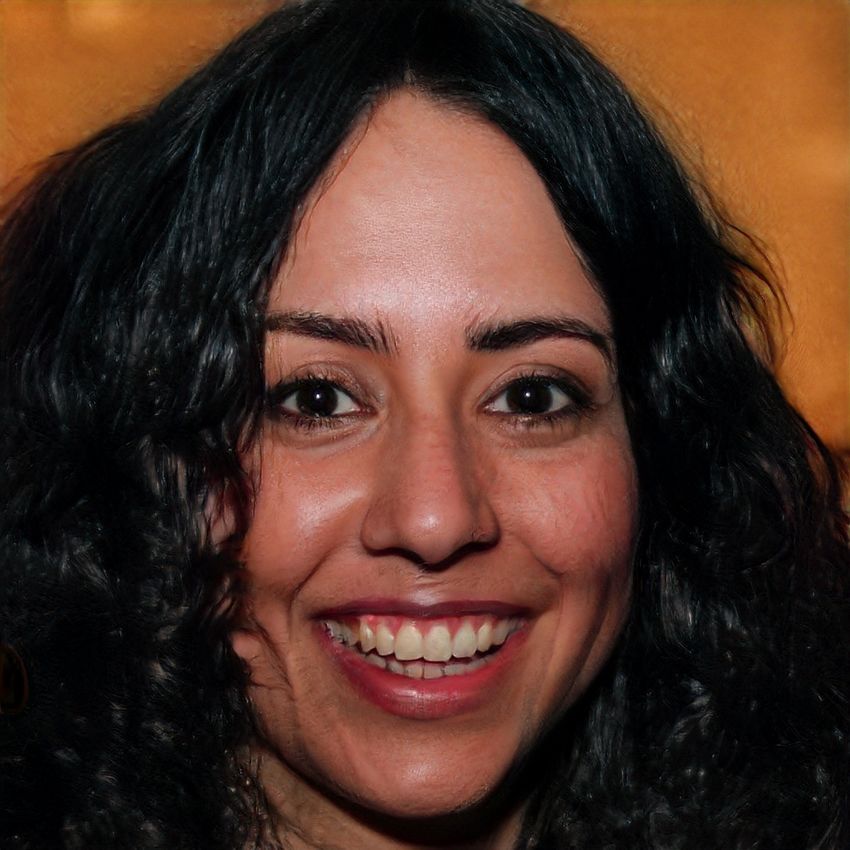
C. Hyperparameters and training details                                               FID                           Path length
                                                                     10                              500
    We build upon the official TensorFlow [1] implemen-
                                                                      9                              400
tation of Progressive GANs by Karras et al. [30], from
which we inherit most of the training details.3 This original         8
                                                                                                     300
setup corresponds to configuration A in Table 1. In particu-          7
lar, we use the same discriminator architecture, resolution-                                         200
                                                                      6
dependent minibatch sizes, Adam [33] hyperparameters,
and exponential moving average of the generator. We en-               5                              100
                                                                                   Full                               Full
able mirror augmentation for CelebA-HQ and FFHQ, but                               resolution                         resolution
                                                                      4                                0
disable it for LSUN. Our training time is approximately one               0   5M   10M 15M 20M 25M         0   5M     10M 15M 20M 25M
                                                                                   Traditional (B)                  Traditional (B)
week on an NVIDIA DGX-1 with 8 Tesla V100 GPUs.
                                                                                   Style-based (F)                  Style-based (F), full
    For our improved baseline (B in Table 1), we make sev-                                                          Style-based (F), end
eral modifications to improve the overall result quality. We
                                                                     Figure 9. FID and perceptual path length metrics over the course
replace the nearest-neighbor up/downsampling in both net-            of training in our configurations B and F using the FFHQ dataset.
works with bilinear sampling, which we implement by low-             Horizontal axis denotes the number of training images seen by the
pass filtering the activations with a separable 2nd order bi-        discriminator. The dashed vertical line at 8.4M images marks the
nomial filter after each upsampling layer and before each            point when training has progressed to full 10242 resolution. On
downsampling layer [64]. We implement progressive grow-              the right, we show only one curve for the traditional generator’s
ing the same way as Karras et al. [30], but we start from 82         path length measurements, because there is no discernible differ-
images instead of 42 . For the FFHQ dataset, we switch from          ence between full-path and endpoint sampling in Z.
WGAN-GP to the non-saturating loss [22] with R1 regular-
ization [44] using γ = 10. With R1 we found that the FID
                                                                     for measuring the separability metric for all generators. We
scores keep decreasing for considerably longer than with
                                                                     will release the pre-trained classifier networks so that our
WGAN-GP, and we thus increase the training time from
                                                                     measurements can be reproduced.
12M to 25M images. We use the same learning rates as
                                                                        We do not use batch normalization [29], spectral nor-
Karras et al. [30] for FFHQ, but we found that setting the
                                                                     malization [45], attention mechanisms [63], dropout [59],
learning rate to 0.002 instead of 0.003 for 5122 and 10242
                                                                     or pixelwise feature vector normalization [30] in our net-
leads to better stability with CelebA-HQ.
                                                                     works.
    For our style-based generator (F in Table 1), we use leaky
ReLU [41] with α = 0.2 and equalized learning rate [30]
for all layers. We use the same feature map counts in our
                                                                     D. Training convergence
convolution layers as Karras et al. [30]. Our mapping net-              Figure 9 shows how the FID and perceptual path length
work consists of 8 fully-connected layers, and the dimen-            metrics evolve during the training of our configurations B
sionality of all input and output activations — including z          and F with the FFHQ dataset. With R1 regularization active
and w — is 512. We found that increasing the depth of                in both configurations, FID continues to slowly decrease as
the mapping network tends to make the training unstable              the training progresses, motivating our choice to increase
with high learning rates. We thus reduce the learning rate           the training time from 12M images to 25M images. Even
by two orders of magnitude for the mapping network, i.e.,            when the training has reached the full 10242 resolution, the
λ0 = 0.01 · λ. We initialize all weights of the convolutional,       slowly rising path lengths indicate that the improvements
fully-connected, and affine transform layers using N (0, 1).         in FID come at the cost of a more entangled representa-
The constant input in synthesis network is initialized to one.       tion. Considering future work, it is an interesting question
The biases and noise scaling factors are initialized to zero,        whether this is unavoidable, or if it were possible to encour-
except for the biases associated with ys that we initialize to       age shorter path lengths without compromising the conver-
one.                                                                 gence of FID.
    The classifiers used by our separability metric (Sec-
tion 4.2) have the same architecture as our discriminator ex-        E. Other datasets
cept that minibatch standard deviation [30] is disabled. We
use the learning rate of 10−3 , minibatch size of 8, Adam               Figures 10, 11, and 12 show an uncurated set of re-
optimizer, and training length of 150,000 images. The                sults for LSUN [62] B EDROOM, C ARS, and C ATS, respec-
classifiers are trained independently of generators, and the         tively. In these images we used the truncation trick from
same 40 classifiers, one for each CelebA attribute, are used         Appendix Bwith ψ = 0.7 for resolutions 42 − 322 . The
                                                                     accompanying video provides results for style mixing and
  3 https://github.com/tkarras/progressive growing of gans           stochastic variation tests. As can be seen therein, in case of

                                                                 9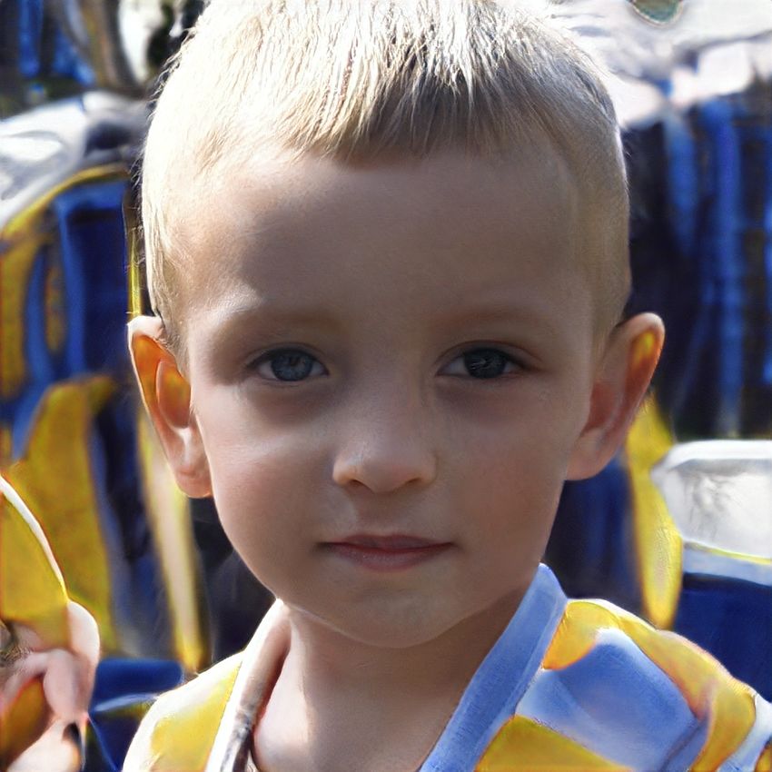
Figure 10. Uncurated set of images produced by our style-based           Figure 11. Uncurated set of images produced by our style-based
generator (config F) with the LSUN B EDROOM dataset at 2562 .            generator (config F) with the LSUN C AR dataset at 512 × 384.
FID computed for 50K images was 2.65.                                    FID computed for 50K images was 3.27.

                                                                         References
B EDROOM the coarse styles basically control the viewpoint                [1] M. Abadi, P. Barham, J. Chen, Z. Chen, A. Davis, J. Dean,
of the camera, middle styles select the particular furniture,                 M. Devin, S. Ghemawat, G. Irving, M. Isard, M. Kudlur,
and fine styles deal with colors and smaller details of ma-                   J. Levenberg, R. Monga, S. Moore, D. G. Murray, B. Steiner,
terials. In C ARS the effects are roughly similar. Stochastic                 P. Tucker, V. Vasudevan, P. Warden, M. Wicke, Y. Yu, and
variation affects primarily the fabrics in B EDROOM, back-                    X. Zheng. TensorFlow: a system for large-scale machine
grounds and headlamps in C ARS, and fur, background, and                      learning. In Proc. 12th USENIX Conference on Operating
interestingly, the positioning of paws in C ATS. Somewhat                     Systems Design and Implementation, OSDI’16, pages 265–
                                                                              283, 2016. 9
surprisingly the wheels of a car never seem to rotate based
on stochastic inputs.                                                     [2] A. Achille and S. Soatto. On the emergence of invari-
                                                                              ance and disentangling in deep representations. CoRR,
                                                                              abs/1706.01350, 2017. 6
   These datasets were trained using the same setup as
                                                                          [3] D. Bau, J. Zhu, H. Strobelt, B. Zhou, J. B. Tenenbaum, W. T.
FFHQ for the duration of 70M images for B EDROOM and                          Freeman, and A. Torralba. GAN dissection: Visualizing
C ATS, and 46M for C ARS. We suspect that the results for                     and understanding generative adversarial networks. In Proc.
B EDROOM are starting to approach the limits of the train-                    ICLR, 2019. 1
ing data, as in many images the most objectionable issues                 [4] M. Ben-Yosef and D. Weinshall. Gaussian mixture genera-
are the severe compression artifacts that have been inherited                 tive adversarial networks for diverse datasets, and the unsu-
from the low-quality training data. C ARS has much higher                     pervised clustering of images. CoRR, abs/1808.10356, 2018.
quality training data that also allows higher spatial resolu-                 3
tion (512 × 384 instead of 2562 ), and C ATS continues to be              [5] A. Brock, J. Donahue, and K. Simonyan. Large scale GAN
a difficult dataset due to the high intrinsic variation in poses,             training for high fidelity natural image synthesis. CoRR,
zoom levels, and backgrounds.                                                 abs/1809.11096, 2018. 1, 3, 8

                                                                    10
[14] H. Drucker and Y. L. Cun. Improving generalization perfor-
mance using double backpropagation. IEEE Transactions on
Neural Networks, 3(6):991–997, 1992. 3
[15] V. Dumoulin, I. Belghazi, B. Poole, A. Lamb, M. Arjovsky,
O. Mastropietro, and A. Courville. Adversarially learned in-
ference. In Proc. ICLR, 2017. 6
[16] V. Dumoulin, E. Perez, N. Schucher, F. Strub, H. d. Vries,
A. Courville, and Y. Bengio. Feature-wise transforma-
tions. Distill, 2018. https://distill.pub/2018/feature-wise-
transformations. 2
[17] V. Dumoulin, J. Shlens, and M. Kudlur. A learned represen-
tation for artistic style. CoRR, abs/1610.07629, 2016. 2
[18] I. P. Durugkar, I. Gemp, and S. Mahadevan. Generative
multi-adversarial networks. CoRR, abs/1611.01673, 2016.
3
[19] C. Eastwood and C. K. I. Williams. A framework for the
quantitative evaluation of disentangled representations. In
Proc. ICLR, 2018. 6
[20] L. A. Gatys, A. S. Ecker, and M. Bethge. Image style transfer
using convolutional neural networks. In Proc. CVPR, 2016.
6
[21] G. Ghiasi, H. Lee, M. Kudlur, V. Dumoulin, and J. Shlens.
Exploring the structure of a real-time, arbitrary neural artistic
stylization network. CoRR, abs/1705.06830, 2017. 2
[22] I. Goodfellow, J. Pouget-Abadie, M. Mirza, B. Xu,
D. Warde-Farley, S. Ozair, A. Courville, and Y. Bengio. Gen-
erative Adversarial Networks. In NIPS, 2014. 1, 3, 9
[23] W.-S. Z. Guang-Yuan Hao, Hong-Xing Yu. MIXGAN: learn-
Figure 12. Uncurated set of images produced by our style-based
ing concepts from different domains for mixture generation.
generator (config F) with the LSUN C AT dataset at 2562 . FID
CoRR, abs/1807.01659, 2018. 2
computed for 50K images was 8.53.
[24] I. Gulrajani, F. Ahmed, M. Arjovsky, V. Dumoulin, and A. C.
Courville. Improved training of Wasserstein GANs. CoRR,
[6] T. Chen, M. Lucic, N. Houlsby, and S. Gelly. On self abs/1704.00028, 2017. 1, 2
modulation for generative adversarial networks. CoRR, [25] M. Heusel, H. Ramsauer, T. Unterthiner, B. Nessler, and
abs/1810.01365, 2018. 3, 8 S. Hochreiter. GANs trained by a two time-scale update rule
[7] T. Q. Chen, X. Li, R. B. Grosse, and D. K. Duvenaud. Isolat- converge to a local Nash equilibrium. In Proc. NIPS, pages
ing sources of disentanglement in variational autoencoders. 6626–6637, 2017. 2
CoRR, abs/1802.04942, 2018. 6 [26] I. Higgins, L. Matthey, A. Pal, C. Burgess, X. Glorot,
[8] X. Chen, Y. Duan, R. Houthooft, J. Schulman, I. Sutskever, M. Botvinick, S. Mohamed, and A. Lerchner. beta-vae:
and P. Abbeel. InfoGAN: interpretable representation learn- Learning basic visual concepts with a constrained variational
ing by information maximizing generative adversarial nets. framework. In Proc. ICLR, 2017. 6
CoRR, abs/1606.03657, 2016. 6 [27] X. Huang and S. J. Belongie. Arbitrary style transfer
[9] E. L. Denton, S. Chintala, A. Szlam, and R. Fergus. Deep in real-time with adaptive instance normalization. CoRR,
generative image models using a Laplacian pyramid of ad- abs/1703.06868, 2017. 1, 2
versarial networks. CoRR, abs/1506.05751, 2015. 3 [28] X. Huang, M. Liu, S. J. Belongie, and J. Kautz. Mul-
[10] G. Desjardins, A. Courville, and Y. Bengio. Disentan- timodal unsupervised image-to-image translation. CoRR,
gling factors of variation via generative entangling. CoRR, abs/1804.04732, 2018. 2
abs/1210.5474, 2012. 6 [29] S. Ioffe and C. Szegedy. Batch normalization: Accelerating
[11] T. Doan, J. Monteiro, I. Albuquerque, B. Mazoure, A. Du- deep network training by reducing internal covariate shift.
rand, J. Pineau, and R. D. Hjelm. Online adaptative curricu- CoRR, abs/1502.03167, 2015. 9
lum learning for GANs. CoRR, abs/1808.00020, 2018. 3 [30] T. Karras, T. Aila, S. Laine, and J. Lehtinen. Progressive
[12] J. Donahue, P. Krähenbühl, and T. Darrell. Adversarial fea- growing of GANs for improved quality, stability, and varia-
ture learning. CoRR, abs/1605.09782, 2016. 6 tion. CoRR, abs/1710.10196, 2017. 1, 2, 7, 8, 9
[13] A. Dosovitskiy, J. T. Springenberg, and T. Brox. Learning to [31] V. Kazemi and J. Sullivan. One millisecond face alignment
generate chairs with convolutional neural networks. CoRR, with an ensemble of regression trees. In Proc. CVPR, 2014.
abs/1411.5928, 2014. 1 8
11[32] H. Kim and A. Mnih. Disentangling by factorising. In Proc. [52] T. Sainburg, M. Thielk, B. Theilman, B. Migliori, and
ICML, 2018. 6 T. Gentner. Generative adversarial interpolative autoencod-
[33] D. P. Kingma and J. Ba. Adam: A method for stochastic ing: adversarial training on latent space interpolations en-
optimization. In ICLR, 2015. 9 courage convex latent distributions. CoRR, abs/1807.06650,
[34] D. P. Kingma and P. Dhariwal. Glow: Generative flow with 2018. 1, 3
invertible 1x1 convolutions. CoRR, abs/1807.03039, 2018. [53] T. Salimans, I. J. Goodfellow, W. Zaremba, V. Cheung,
3, 8 A. Radford, and X. Chen. Improved techniques for training
GANs. In NIPS, 2016. 7
[35] D. P. Kingma and M. Welling. Auto-encoding variational
bayes. In ICLR, 2014. 6 [54] J. Schmidhuber. Learning factorial codes by predictability
minimization. Neural Computation, 4(6):863–879, 1992. 6
[36] K. Kurach, M. Lucic, X. Zhai, M. Michalski, and S. Gelly.
[55] R. Sharma, S. Barratt, S. Ermon, and V. Pande. Improved
The gan landscape: Losses, architectures, regularization, and
training with curriculum gans. CoRR, abs/1807.09295, 2018.
normalization. CoRR, abs/1807.04720, 2018. 1
3
[37] S. Laine. Feature-based metrics for exploring the latent space
[56] K. Shoemake. Animating rotation with quaternion curves. In
of generative models. ICLR workshop poster, 2018. 1, 6
Proc. SIGGRAPH ’85, 1985. 7
[38] Y. Li, C. Fang, J. Yang, Z. Wang, X. Lu, and M.-H. Yang. [57] A. Siarohin, E. Sangineto, and N. Sebe. Whitening and col-
Universal style transfer via feature transforms. In Proc. oring transform for GANs. CoRR, abs/1806.00420, 2018.
NIPS, 2017. 2 2
[39] Y. Li, N. Wang, J. Liu, and X. Hou. Demystifying neural [58] K. Simonyan and A. Zisserman. Very deep convolu-
style transfer. CoRR, abs/1701.01036, 2017. 6 tional networks for large-scale image recognition. CoRR,
[40] M. Lucic, K. Kurach, M. Michalski, S. Gelly, and O. Bous- abs/1409.1556, 2014. 6
quet. Are GANs created equal? a large-scale study. CoRR, [59] N. Srivastava, G. Hinton, A. Krizhevsky, I. Sutskever, and
abs/1711.10337, 2017. 1 R. Salakhutdinov. Dropout: A simple way to prevent neu-
[41] A. L. Maas, A. Y. Hannun, and A. Ng. Rectifier nonlin- ral networks from overfitting. Journal of Machine Learning
earities improve neural network acoustic models. In Proc. Research, 15:1929–1958, 2014. 9
International Conference on Machine Learning (ICML), vol- [60] T. Wang, M. Liu, J. Zhu, A. Tao, J. Kautz, and B. Catanzaro.
ume 30, 2013. 9 High-resolution image synthesis and semantic manipulation
[42] M. Marchesi. Megapixel size image creation using genera- with conditional GANs. CoRR, abs/1711.11585, 2017. 3
tive adversarial networks. CoRR, abs/1706.00082, 2017. 3, [61] T. White. Sampling generative networks: Notes on a few
8 effective techniques. CoRR, abs/1609.04468, 2016. 7
[43] L. Matthey, I. Higgins, D. Hassabis, and A. Lerch- [62] F. Yu, Y. Zhang, S. Song, A. Seff, and J. Xiao. LSUN: Con-
ner. dsprites: Disentanglement testing sprites dataset. struction of a large-scale image dataset using deep learning
https://github.com/deepmind/dsprites-dataset/, 2017. 6 with humans in the loop. CoRR, abs/1506.03365, 2015. 9
[44] L. Mescheder, A. Geiger, and S. Nowozin. Which train- [63] H. Zhang, I. Goodfellow, D. Metaxas, and A. Odena.
ing methods for GANs do actually converge? CoRR, Self-attention generative adversarial networks. CoRR,
abs/1801.04406, 2018. 1, 3, 9 abs/1805.08318, 2018. 3, 9
[45] T. Miyato, T. Kataoka, M. Koyama, and Y. Yoshida. Spectral [64] R. Zhang. Making convolutional networks shift-invariant
normalization for generative adversarial networks. CoRR, again, 2019. 2, 9
abs/1802.05957, 2018. 1, 9 [65] R. Zhang, P. Isola, A. A. Efros, E. Shechtman, and O. Wang.
[46] T. Miyato and M. Koyama. cGANs with projection discrim- The unreasonable effectiveness of deep features as a percep-
inator. CoRR, abs/1802.05637, 2018. 3 tual metric. In Proc. CVPR, 2018. 6, 7
[47] G. Mordido, H. Yang, and C. Meinel. Dropout-gan: Learn-
ing from a dynamic ensemble of discriminators. CoRR,
abs/1807.11346, 2018. 3
[48] S. Mukherjee, H. Asnani, E. Lin, and S. Kannan. Cluster-
GAN : Latent space clustering in generative adversarial net-
works. CoRR, abs/1809.03627, 2018. 3
[49] D. J. Rezende, S. Mohamed, and D. Wierstra. Stochastic
backpropagation and approximate inference in deep genera-
tive models. In Proc. ICML, 2014. 6
[50] K. Ridgeway. A survey of inductive biases for factorial
representation-learning. CoRR, abs/1612.05299, 2016. 6
[51] A. S. Ross and F. Doshi-Velez. Improving the adversarial
robustness and interpretability of deep neural networks by
regularizing their input gradients. CoRR, abs/1711.09404,
2017. 3
12You can also read